Baycrest Research Division - Enriching Care, Enhancing Knowledge, Enlightening Minds

Partial Least Squares (PLS), which was first introduced to the neuroimaging community in 1996 (McIntosh et al., 1996), has proven to be a robust method for describing the relationship between signal changes in brain and a set of exogenous variables (i.e. task demands, performance, or activity in other brain regions).

PLS Applications include a Graphic User Interface - GUI application and a Command-Line computation application. Both applications must be kept under the same parent folder, and their folder names (i.e. plsgui and plscmd) can not be changed.

If you would like to use GUI interface, path to plsgui folder must be manually added in MATLAB command window. When you run PLS analysis, computation part in plscmd folder will automatically be called internally. You only need to type plsgui, and a GUI interface will be driven by messages from your mouse and keyboard inputs. As an alternative, you can also run GUI interface unattendedly with Batch Process.

Command-Line PLS (see Appendix B) pls_analysis is the core computation application of PLS. All PLS computations in the GUI will resort to pls_analysis application. If you would like to use Command-Line PLS alone, you can manually add a path to plscmd folder in MATLAB command window. However, keep in mind that its result is only part of GUI result, and cannot be displayed under GUI interface.

PLS Applications are zipped into Pls.zip file, and can be downloaded from the Download Files web page.

This User Guide only intends to show HOW to use PLS Applications for those users who have already understood the PLS method. If PLS is new to you and you want to know WHY PLS Applications are designed this way, please refer to the relevant articles listed at the bottom.

2. PLS Applications Support

Here are the links to some useful web pages for PLS Applications:

For on-line help: http://pls.rotman-baycrest.on.ca/UserGuide.htm
To download files: http://pls.rotman-baycrest.on.ca/source
For the latest update: http://pls.rotman-baycrest.on.ca/whatsnew.txt
Frequently asked questions: http://pls.rotman-baycrest.on.ca/FAQ.txt
To post questions: http://www.rotman-baycrest.on.ca/index.php?section=105
Journal Articles: http://www.rotman-baycrest.on.ca/index.php?section=101

3. System Requirement

PLS Applications are able to run on all versions of MATLAB from 5.3.1 and above, on all the platforms. Because PLS Applications are based on all the information from the raw images, we suggest that you would better add as much memory as your system can support. If you use MATLAB Version 7 (R14) and above, all modules except ERP will automatically take advantage of MATLAB's single precision math operation feature.

If you do not have powerful system with lots of memories, you might want to consider re-sampling the raw images to larger voxel size. When you increase the voxel size, the total number of voxel is reduced, and the dataset size is also reduced.

4. Getting Started

In MATLAB command window, type plsgui, and you will see PLS start window (Figure 1).

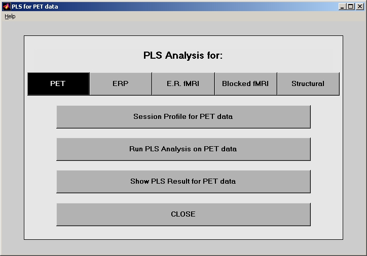
Figure 1

Buttons on top row stand for PLS modules, and you must select a module first. Below the top row, there are 4 buttons, which indicate the basic flow of an experiment: Session Profile, Run PLS Analysis, Show PLS Result, and CLOSE. This User Guide will use the basic flow as a thread for further introduction. Please follow the flow from top to bottom.

Caution: Please remember that result file must be kept in the same folder as sessiondata files that are used when creating the result (e.g. sessiondata.mat, data.mat, etc.). The reason is to prevent from storing path in the result file, so that those files can be moved around without problem.

Please follow the steps below to learn how to use PLS Applications.

5. Session Profile

PLS session profile need to be created before running analysis. The file name of PLS session profile should look like this: prefix_MODULEsessiondata.mat. However, in PLS version 5.x or earlier, old file pair session.mat / datamat.mat were used. In order to make the version change seamless, a program session2sessiondata.m is provided, which can convert old file pair into a single sessiondata.mat file. For more information, please type: help session2sessiondata in MATLAB command window. For Structural MRI and ERP modules, sometimes there can be more datamat.mat files point to one session.mat file. In this case, simply copy the datamat.mat file to sessiondata.mat file, and keep the prefix of datamat.mat file. However, this does not apply to other modules.

In order to create session profile, raw data (scan images, ERP data etc.) must be saved in following ways before launching PLS Applications.

For PET and ERP modules, each subject should have its own folder containing PET scan images or ERP data of all conditions for this subject, and all subjects' folders should under the same (parent) folder.

For E.R.fMRI and Blocked fMRI modules, each run should have its own folder containing MRI scan images of all conditions for this run. All image file names in the run folder should be sorted in alphabetic ascend order that represents scans of this run in time series sequence.

For Structural MRI module, all subjects with all conditions are kept in a single folder. The naming convention for raw data files in Structural module is critically important, which will be introduced in Creating Structural MRI sessiondata file section.

For PET, Structural MRI, E.R.fMRI and Blocked fMRI data, PLS can use both Aanalyze format images (Mayo Clinic) and NIfTI format images (National Institutes of Health). For ERP (including MEG) data, PLS can read tab (or space) delimited text data files from any system, as well as some of the binary data files, such as NeuroScan average data, ANT's average data, EGI's simple-binary data.

All raw data must be properly pre-processed (registered to the same brain template, smoothed with some filters, etc.) prior to using PLS.

5.1. Creating PET sessiondata file

In PLS start window, click PET button and it will be highlighted. Then click Session Profile for PET data button below, the session window will open (Figure 2).

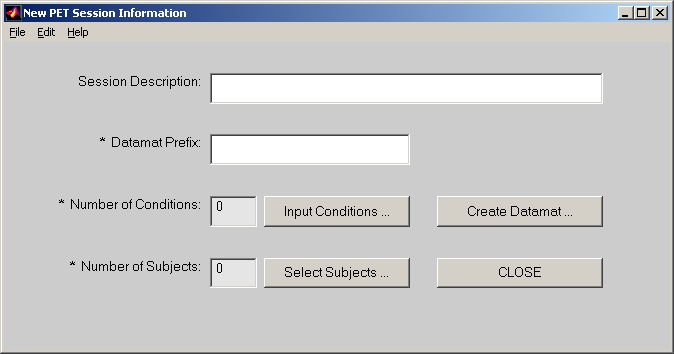
Figure 2

In the session window, Session Description is an optional field.

Datamat Prefix is used to compose sessiondata file name. For example, if you put demo in this field, the sessiondata file will become demo_PETsessiondata.mat.

Click Input Conditions button, and add condition names one by one into the Edit Condition window. When you click DONE, Number of Conditions will show how many conditions you have selected.

As we mentioned above, all PET scan images for each subject should be kept in one folder, and all subjects for one analysis should be under a single folder. If a PET file is in NIfTI image and contains multiple-scans, it must be expanded to multiple single-scan files with MATLAB program expand_nii_scan.m that is included in PLS Applications.

Now, click Select Subjects button, and the Edit Subject Directory window will open (Figure 3).

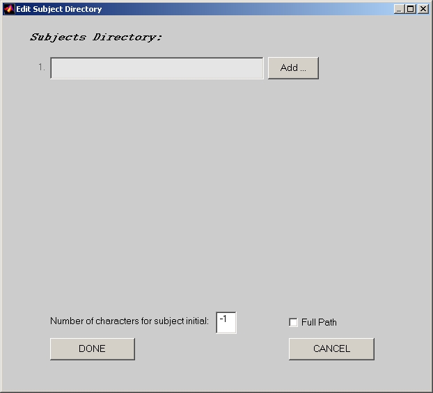
Figure 3

There is an edit box called Number of character for subject initial in the Edit Subject Directory window. Change the value from -1 to the length of subject initial if your subject files follow the following Consistent Naming Across Subjects rule:

All subject files consist 2 parts, subject initial part and condition name part. e.g. SubjInit1_CondName1
Across all subject directories, the condition name part should be the same for the same condition.
Within each subject directory, the subject initial part should be the same for all conditions within this subject.

Click Add button, and the Subject Directory Detail window will open (Figure 4).

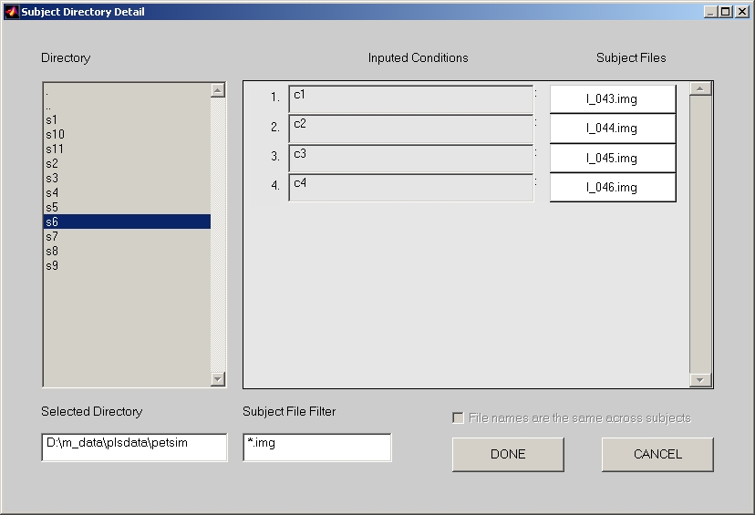
Figure 4

If your subject files follow the Consistent Naming Across Subjects rule, follow the steps below:

Enter the length of the subject initials in the Number of Characters for subject initial box in previous window.
Select one of subjects that will be used in this datamat group (Note: Remember to only select 1 subject this time).
If you have Consistent Naming Across Subjects, you will notice that File names are the same across subjects check box is checked. Uncheck it to disable this feature.
Go to right hand side, select correct subject files that match the inputted conditions at their left side. Make sure that no subject file can be duplicated.
If you have multiple subjects in this group, you can now select the rest of subjects by holding Shift or Ctrl key combination while selecting (Note: You cannot do so before this step).
Click Done button when you finish, and return to Session Information window.

If your subject files do not follow the Consistent Naming Across Subjects rule, you can still follow the steps above. However, you will have to go to Edit Subject Directory window, click Edit button, and select correct subject files to match the inputted conditions for each single subject.

Go back to PET session window, and click Create Datamat button to open Create PET Datamat window.

There are two ways to define brain region:

Use pre-defined brain region image file, which should have the same dimension and orientation as any PET scan images in the subjects. The intensity of the brain region image should be either 0 or 1 (binary image), where 1 stands for the brain region.
Define brain region automatically with a threshold. If a voxel's intensity is greater than the threshold multiplied by the maximum intensity, it is considered as a brain voxel. Since any voxel intensity that is less than the threshold multiplied by the maximum intensity will be treated non-brain region, we require that the minimum of image intensity should be no less than 0.

If Normalize data with volume mean is checked, datamat value will be the stacked volume intensity divided by the average intensity for each volume; otherwise, datamat value will just be the stacked volume intensity. Please be aware that by default Normalize data with volume mean is checked for PET data.

Click Merge Conditions button to combine two or more conditions together to a new condition by averaging them.

You can verify image orientation by clicking Check image orientation button. If you believe that the image orientation is wrong, you can click Re-orient button to make change.

Now, click Create button to generate PET sessiondata file.

5.2. Creating ERP sessiondata file

In PLS start window, click ERP button and it will be highlighted. Then click Session Profile for ERP data button below, the session window will open (Figure 5).

Figure 5

In the session window, Session Description is an optional field.

Datamat Prefix is used to compose file names for ERP sessiondata file and ERP data file. For example, if you put demo in this field, demo_ERPsessiondata.mat will be the ERP sessiondata file name and demo_ERPdata.mat will be the ERP data file name.

Digitization Interval is the inverse of sampling rate. It is in millisecond (default is 2ms).

Prestim Baseline shows how early the time points start before stimulus is applied to a subject. It is also in millisecond (default is 0), and the value should be less than or equal to 0.

Click Input Conditions button, and add condition names one by one into the Edit Condition window. When you click DONE, Number of Conditions will show how many conditions you have selected.

As we mentioned above, all ERP raw data for each subject should be kept in one folder, and all subjects for one analysis should be under a single folder. Now, click Select Subjects button to select and edit subjects in subject folder. The steps are the same as those in PET.

If ERP data is a delimited text file, each row usually stands for an electrode channel and each column usually stands for a time point. However, column can be used for channel if Channel in column check box is selected.

In order to match row (or column) of ERP data with electrode channel name, you need to click Edit Channel Order button. If your ERP data are binary files, an additional Select an EEG format window will popup, and you can select the proper vendor name and machine format. No matter your ERP data are binary files or plain text files, you will end up with an Edit Channel Order window (Figure 6).

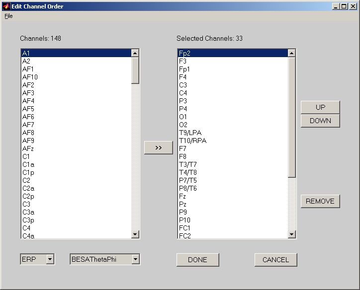
Figure 6

What on the left panel of Edit Channel Order window is a complete channel name list based on the two system boxes below that panel. You can either manually select and add them to the right panel (you only need to do this once), or load from an existing channel list text file that you have saved before through File menu (much more conveniently). Click DONE when finish, and Number of Channels will show how many channels you selected.

In the lower left corner of the Edit Channel Order window, you can select different scalp electrode location systems and sub-systems. When you change the system or sub-system, you can notice that channel name list on the left panel of Edit Channel Order window changes.

What if you have a scalp electrode system that can not be found in the system boxes (e.g. Standard 10-20 EEG System with 19 cap electrodes)? Please follow the steps below to add your own system:

Put all electrode names on a piece of grid paper, and make sure that they are spatially located appropriately.
Select an origin for XY coordinates. You can pick any point (on or off any electrode) as your origin. For example, Cz is a good selection, the most lower left grid is also a good selection.
Use a ruler (or count the grid) to measure the x and y location from the origin.
Assign your channel names to chan_nam variable, and assign x and y location to chan_loc variable (x is at left, and y is at right). The rows of chan_nam must match the rows of chan_loc variable, which stand for the channels. Like this:

chan_nam=[

�� 'Fp1'

�� 'Fp2'

�� 'F7 '

�� 'F3 '

�� 'Fz '

�� 'F4 '

�� 'F8 '

�� 'T7 '

�� 'C3 '

�� 'Cz '

�� 'C4 '

�� 'T8 '

�� 'P7 '

�� 'P3 '

�� 'Pz '

�� 'P4 '

�� 'P8 '

�� 'O1 '

�� 'O2 '�� ]

chan_loc=[

�� -3� 10

�� 3�� 10

�� -8� 6

�� -5� 7

�� 0�� 8

�� 5�� 7

�� 8�� 6

�� -10 0

�� -7� 0

�� 0�� 0

�� 7�� 0

�� 10� 0

�� -8� -6

�� -5� -7

�� 0�� -8

�� 5�� -7

�� 8�� -6

�� -3� -10

�� 3�� -10�� ]

Assume that your current folder is the one that you will save sessiondata & result files, then run:

save erp_loc_besa148 chan_loc chan_nam

Now you have your own electrode system in Edit Channel Order window if you select ERP/BESAThetaPhi system.

Obviously, here the ERP/BESAThetaPhi system now represents your own system instead of the real ERP/BESAThetaPhi system from PLS Applications. If you want to restore the real ERP/BESAThetaPhi system from PLS Applications, you can choose a different folder for different experiment, or simply remove erp_loc_basa148.mat file in this folder.

ERP module is very different from other modules, because of its small raw dataset. For this reason, we put all subjects with all conditions into one file, which we call it ERP data file. Then you can have several ERP sessiondata files point to one ERP data file, and each of those ERP sessiondata file is part (or all) of this ERP data. ERP data file is generated at the same time when you generate ERP sessiondata file.

Go back to ERP session window, and click Create Datamat button to open Create Datamat window (Figure 7).

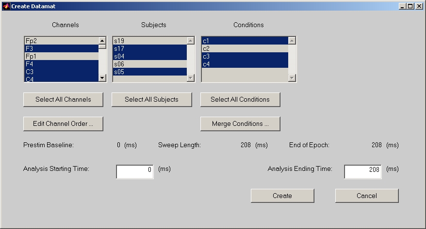
Figure 7

In this window, you can deselect Channels, Subjects and Conditions. The Select All button below let you easily reset to the default all selected.

Edit Channel Order here can also let you modify the channel name, but we suggest that you had better to do it in the session window, since any change here will not be saved in the sessiondata file.

Click Merge Conditions button to combine two or more conditions together to a new condition by averaging them.

You can also specify time-points range for ERP datamat, which must be within Prestim Baseline and End of Epoch.

Now, click Create button to generate ERP sessiondata file and ERP data file.

5.3. Modifying ERP sessiondata file and saving to a different file name

In ERP session window, click Modify Datamat button, and select an ERP sessiondata file that you are going to modify. The Modify Datamat window opens with ERP Amplitude plot window. As you can see that ERP Modify Datamat window is very close to ERP Create Datamat window. There are only two differences, which are:

Merge Conditions button is removed, since you cannot change ERP data file by modifying ERP sessiondata file.
Save Datamat As field is added. This way, we only need to create a single ERP sessiondata file, and then modify it (e.g. select different subjects etc.) and save it to a different ERP sessiondata file name.

Click Modify button to save the modified sessiondata file, and the ERP Amplitude plot will immediately reflect the new sessiondata file.

5.4. Creating E.R.fMRI sessiondata file

In PLS start window, click E.R.fMRI button and it will be highlighted. Then click Session Profile for E.R.fMRI data button below, the session window will open (Figure 8).

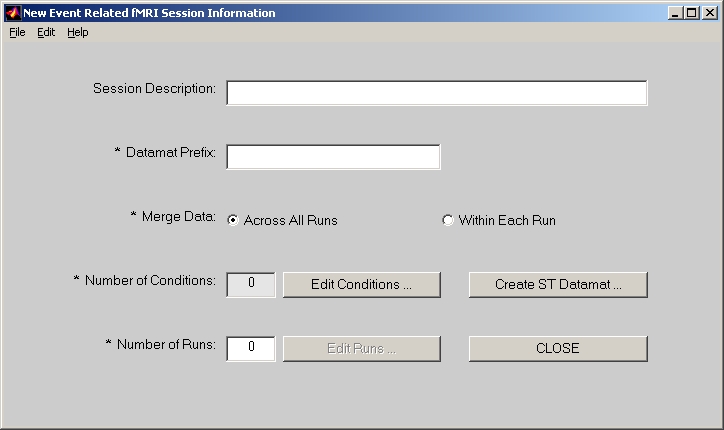
Figure 8

In the session window, Session Description is an optional field.

Datamat Prefix is used to compose sessiondata file name. For example, if you put demo in this field, the sessiondata file will become demo_fMRIdatamat.mat.

Datamat can be merged Across All Runs or Within Each Run only. If Across All Runs is selected (by default), data will be averaged together across all runs for the same condition names. If Within Each Runs is selected, the same condition name in different runs will be treated as different conditions. So the actual conditions will be automatically expand to something like Run1Cond1, Run1Cond2, �, Run2Cond1, etc.

Click Edit Conditions button, and add condition names one by one into the Edit Condition window. Besides Condition Name field, there are two more fields: Relative Ref. Scan Onset and Number of Reference Scans. They are only used if you select Normalize data with ref. scans check box in Generate ST Datamat window. Relative Ref. Scan Onset refers the offset of the first reference scan from the first scan of each onset. Negative value means that reference scan starts before the first scan of each onset. By default, it is 0. Number of Reference Scans means how many scans after the first reference scan will be averaged together to become a reference scan. By default, it is 1, which means that only 1 scan is used for reference scan. When you click DONE, Number of Conditions will show how many conditions you selected.

Number of Runs field must be entered first before clicking Edit Runs. It indicates how many runs of data will be used. Each run of data must be kept in a separate folder.

Click Edit Runs button to open Run Information window (Figure 9):

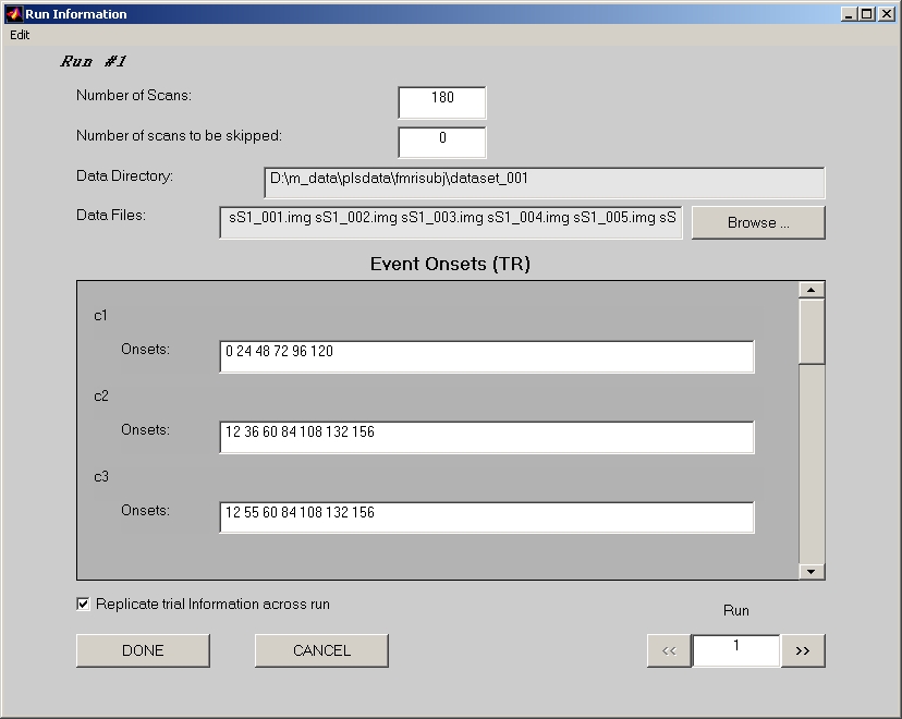
Figure 9

Number of Scans field must be specified first in this window.
If Number of scans to be skipped is not 0, the first several scans in this run to be skipped should not be included in the Data Files, and Number of Scans should reflects the actual number of un-skipped scans. The onset number in the fields below still starts from the very first scan of this run. If the onsets that you entered are within the skipped scans, they will be excluded when the datamat is created.
Click Browse to open Select Data Files window. Once click DONE in Select Data Files window, Data Directory field and Data Files field in the Run Information window are both filled.
Fill Onsets fields condition by condition. Please be aware that the scan starts from 0, and unit is TR or scan, not second. i.e. If you put number 10, it refers the 11th scan image you selected.
If you have many onset numbers in a field, we suggest you to prepare them in text files. One text file for each run, each line stands for a condition, and all onsets for that condition are separated by a space and listed on that condition line. Click Load Onsets from a text file for this run under Edit menu to let the PLS applications fill the onset numbers for you. Click Save Onsets to a text file for this run will save the current filled numbers to a text file.
If Replicate trial information across run is selected (by default), the onset number will stay the same while you traverse from run to run.
If you decide to completely drop this run, you can click Delete under Edit menu to delete this run.

Click >> button to go to next run, and repeat the steps above for all the runs.

Go back to E.R.fMRI session window, and click Create ST Datamat button to open Generate ST Datamat window (Figure 10).

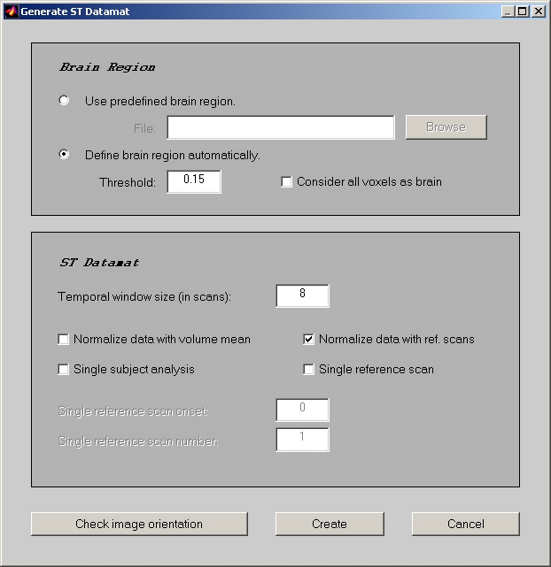
Figure 10

There are two ways to define fMRI brain region, and they are the same as two ways to define PET brain region. Since any intensity of voxel that is less than the threshold of maximum intensity will be treated non-brain region, we require that the minimum of image intensity should be no less than 0.

Temporal window size refers to the length of hemodynamic period, and unit is TR or scan. e.g. If the length of hemodynamic period is 16 seconds and each TR is 2 seconds, then Temporal window size is 8 scans.

If Normalize data with ref. scans is checked, datamat will be normalized by the selected ref. scans. Please be aware that by default Normalize data with ref. scans is selected for both E.R.fMRI and Blocked fMRI data to prevent huge DC offset (low frequency noise).

Single subject analysis is only used to analyze single subject with very few onsets. If this check box is selected, each onset block will be stacked as a separate volume. So, datamat will only be averaged within each onset block, rather than within each condition.

Single reference scan will use the reference scan below for all the scans in the datamat, which will replace whatever Relative Ref. Scan Onset and Number of Reference Scans that you set in the Edit Condition window. It is also only used when you select the Normalize data with ref. scans check box. In Single reference scan onset edit box below, you enter an absolute reference scan onset, instead of a relative reference scan onset.

Now, click Create button to generate E.R.fMRI sessiondata file.

5.5. Creating E.R.fMRI sessiondata file with user defined HRF

In PLS start window, click Blocked fMRI button and it will be highlighted. Then click Session Profile for Blocked fMRI data button below, the session window will open (Figure 11).

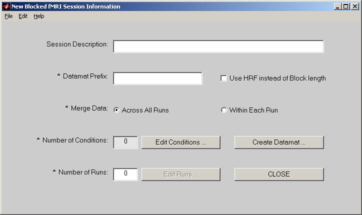
Figure 11

This window is very similar to the regular E.R.fMRI session window, except that there is a check box called Use HRF instead of Blocked Length. If you check this box, your sessiondata file is for E.R.fMRI with user defined HRF; if you uncheck this box, your sessiondata file will become Blocked fMRI, which will be described below. Once you make the decision, it cannot be changed. If you really want to change, you will have to make a new sessiondata file.

Like regular E.R.fMRI session window, click Edit Runs button to open Run Information window (Figure 12):

Figure 12

This is also very similar to the regular E.R.fMRI Run Information window, except that there is one more field under Onsets, which is called Duration, and is used for epoch-related response. If your experiment is only for event-related response, just enter 0.

Go back to session window, click Create Datamat button to open the Generate Datamat window (Figure 13).

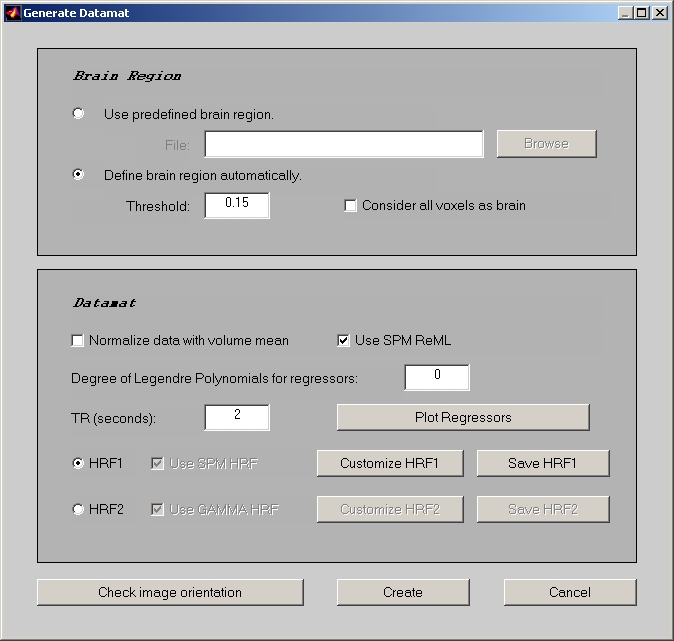
Figure 13

The Brain Region section is exactly the same as the regular E.R.fMRI, but the Datamat section is completely different.

If Use SPM ReML is checked, you are using the feature that is copied from SPM to remove the voxel outliers over the run. It is a temporal whitening function using restricted maximum likelihood estimation.

Degree of Legendre Polynomials for regressors is used to define the baseline regressor(s). By default, it is 0, which provides a single column of all ones.

You must enter the length of TR (in seconds) in order to define the HRF.

Then, you have two options to define the HRF:� HRF1 & HRF2. In HRF1, TR will be further divided when calculating design matrix. By default, it will use HRF model from SPM, since most codes are copied from SPM. In HRF2, TR is always the smallest unit when calculating design matrix. By default, it will use GAMMA HRF from AFNI. In both case, you can click Customize HRF to modify the model, and click Save HRF to save the model.

When you click Plot Regressors, the entire hemodynamic response across the run will be displayed. This is actually the convolution result between HRF and event (or epoch), which is sometimes also called design matrix.

Now, click Create button to generate E.R.fMRI sessiondata file with user defined HRF.

5.6. Creating Blocked fMRI sessiondata file

Creating Blocked fMRI sessiondata file is almost the same as Creating E.R.fMRI sessiondata file with user defined HRF. However, don�t check Use HRF instead of Blocked Length check box, which is for E.R.fMRI with user defined HRF.

5.7. Creating Structural sessiondata file

In PLS start window, click Structural button and it will be highlighted. Then click Session Profile for Structural data button below, the session window will open (Figure 14).

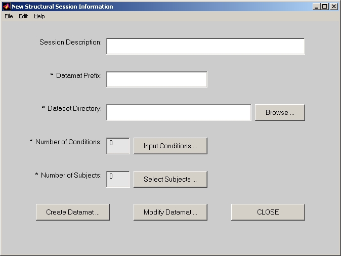
Figure 14

In the session window, Session Description is an optional field.

Datamat Prefix is used to compose file names for Structural sessiondata file and Structural data file. For example, if you put demo in this field, demo_STRUCTdatamat.mat will be the Structural sessiondata file name and demo_STRUCTdata.mat will be the Structural data file name.

Dataset Directory is where raw data of all subjects with all conditions are kept. The file name convention for dataset file here is criticlly important. All those file names have to be composed in three parts: subject part followed by condition part followed by dataset format part. For the same subject, different conditions should have the same subject part; for the same condition, different subjects should have the same condition part; the dataset format part should be either .nii or .img/hdr. For example, assuming that there are subjects "s1_" "s2_" "s3_" with conditions "wm" "gm" and format "nii", there must be at least six files in this folder: s1_wm.nii, s2_wm.nii, s3_wm.nii, s1_gm.nii, s2_gm.nii, s3_gm.nii.

Click Input Conditions button, and add condition names one by one into the Edit Condition window (Figure 15). Besides Condition Name field, there is one more field: Condition Filter. You must enter wildcard (e.g. *wm.nii) to distinguish files with different conditions. When you click DONE, Number of Conditions will show how many conditions you have selected.

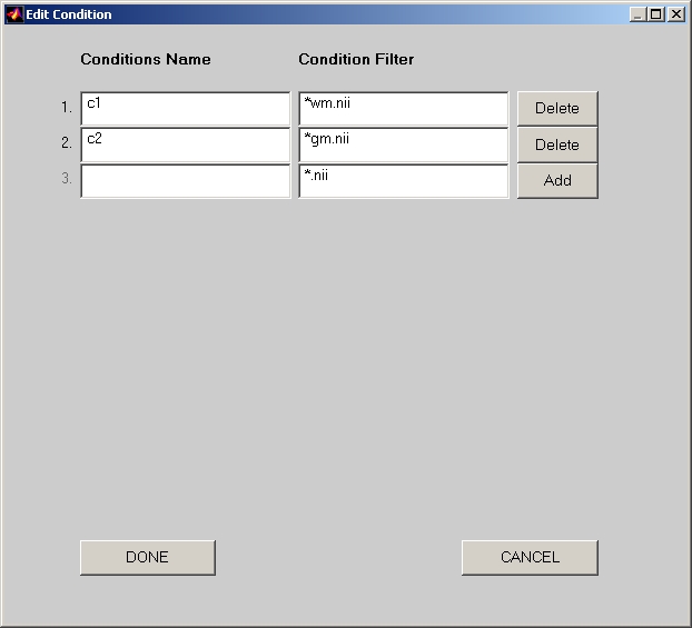
Figure 15

Click Select Subjects button, and the Edit Subject Directory window will open (Figure 3). Now, click Add button, and the Subject Directory Detail window will open (Figure 16). You can select one or more subjects for this datamat group. By default, subject name is the dataset file name without condition filter part. If you feel the subject name too long, you can always change it in the Edit Subject Directory window.

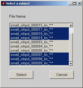
Figure 16

Like ERP module, we put all subjects with all conditions into one file, which we call it Structural data file. Then we have several Structural sessiondata files point to one Structural data file, and each of those Structural sessiondata file is part (or all) of this Structural data. Structural data file is generated at the same time when you create Structural sessiondata file.

In Structural session window, click Create Datamat button and it opens Create Datamat window (Figure 17).

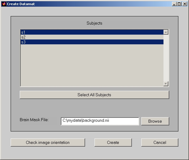
Figure 17

In this window, you can deselect the subjects. The Select All Subjects button below let you easily reset to the default all selected.

In Brain Mask File field, you must provide a pre-defined brain region image file.

Now, click Create button to generate Structural sessiondata file and Structural data file.

5.8. Modifying Structural sessiondata file and saving to a different name

In Structural session window, click Modify Datamat button, and select a Structural sessiondata file that you are going to modify. The Modify Datamat window opens. As you can see that Structural Modify Datamat window is very close to Structural Create Datamat window. There are only three differences, which are:

Brain Mask File field is removed, since you cannot change Structural data file by modifying Structural sessiondata file.
Check image orientation button is removed for the same reason.
Save Datamat As field is added. This way, we only need to create a single Structural sessiondata file, and then modify it (e.g. select different subjects etc.) and save it to a different Structural sessiondata file name.

Click Modify button to save the modified sessiondata file.

6. Run PLS analysis

The purpose of performing PLS analysis on neuroimaging data is to obtain result data that can better interpret the brain activities and other brain statistical information, which can include singular values, singular vectors, etc. The internal procedures of an analysis includes:

Stack datamat in the format of subject within condition within group. For Behavior PLS and Multiblock PLS, behavior data should also be stacked in this way.
Generate a covariance or correlation matrix from the stacked datamat (and stacked behavior data).
Decompose the covariance or correlation matrix to compute the singular vectors.
Run permutation for significance test (optional).
Run bootstrap for reliability test (optional).

In PLS start window, select a module and then click Run PLS Analysis button below, the analysis window will open (Figure 18).

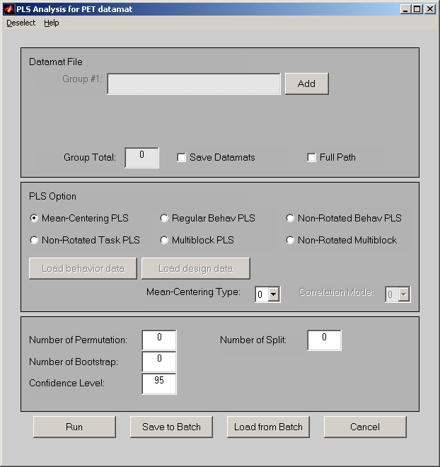
Figure 18

The PLS analysis window is almost identical across all modules. However, there are still some slight differences. e.g. For PET, ERP and Structural module, each group only contains one sessiondata file. For E.R.fMRI and Blocked fMRI module, each group can contain more than one sessiondata file.

In the analysis window, group files must be added first. For PET, ERP and Structural module, click Add button to select a sessiondata file for each group. For E.R.fMRI and Blocked fMRI module, click Add button will open a Select Session Profiles window (Figure 19) for a group.

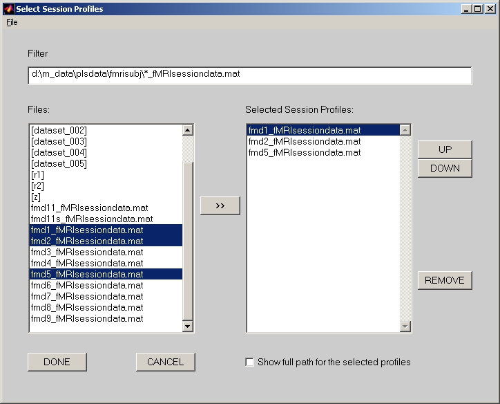
Figure 19

Highlight E.R.fMRI and Blocked fMRI sessiondata files for this group, and click >> button to add them into the right panel. You can save this selection by clicking Save to a text file under File menu of Select Session Profiles window. Next time, you do not need to select those sessiondata files again. You can click Load from a text file under File menu of this window, and those selections you selected will be loaded in this window.

The Group Total in PLS analysis window will display how many groups you selected. The Save Datamats check box is only selected if you want to save the stacked datamat. We advise regular users not to select this check box, since it will make the size of result file much larger. After all group files are added, you also have an option to remove some conditions by clicking Deselect conditions under Deselect menu. You do not have to do this unless it is necessary.

Now you have to select one of the PLS options:

If you choose Mean-Centering Task PLS option, the data will be mean-centered before being decomposed with singular value decomposition (SVD) to singular values, singular vectors, etc. In Mean-Centering Task PLS, Non-Rotated Task PLS, Multiblock PLS and Non-Rotated Multiblock PLS, Mean-Centering Type can be selected, which is set to 0 by default.

If you choose Non-Rotated Task PLS, No-Rotated Behav PLS or Non-Rotated Multiblock PLS, priori contrast is used to restrict the patterns derived from PLS. So you also need to provide a contrast in order to run this analysis. Click Load design data button below, and the Contrast window (Figure 20) will open.

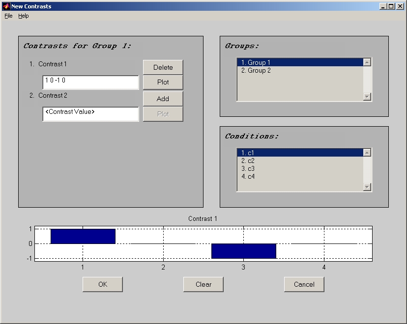
Figure 20

In the contrast window, field Contrast 1 stands for 1st contrast, and field Contrast 2 stands for 2nd contrast, etc. The 1st value in each contrast field is for the 1st selected condition, and the 2nd one is for the 2nd selected condition, etc. Click Add button beside contrast field to input the contrast value, and lick Plot button to display bar graph of this contrast. If you have more than 1 group, you also have to fill all contrast fields for all groups. Highlight different group name in Groups panel to switch groups.

By clicking Load or Save item under File menu of the contrast window, you can load a contrast from a text file or save it to a text file.

For Regular Behav PLS, Non-Rotated Behav PLS, Multiblock PLS or Non-Rotated Multiblock PLS, you must have at least 3 subjects in order to generate proper correlation matrix and run PLS properly. In these PLS options, you can select Correlation Mode which is set to 0 by default. In addition, behavior data must be provided to compute the correlation matrix between the measures and the datamat. Each column in the behavior data stands for one behavior measure, and is separated by a space. The rows should be arranged in the order of subjects in selected conditions in groups, which is the same as datamat row order.

For example, let's say you have group1 and group2 with condition1, and condition2. In group1, you have 2 subjects, and in group2 you have 3 subjects. Here is the order of the behavior file:

group1�� condition1�� subject1

group1�� condition1�� subject2

group1�� condition2�� subject1

group1�� condition2�� subject2

group2�� condition1�� subject1

group2�� condition1�� subject2

group2�� condition1�� subject3

group2�� condition2�� subject1

group2�� condition2�� subject2

group2�� condition2�� subject3

In Multiblock PLS, some conditions in behavior block can also be deselected, and there is no behavior data for the deselected conditions. In that case, please pad any number (e.g. 0) to the missing value in behavior data for those deselected conditions, which will be skipped during the analysis.

To input behavior data for PLS Applications, click Load behavior data button, and the Edit Behavior Data window will open (Figure 21).

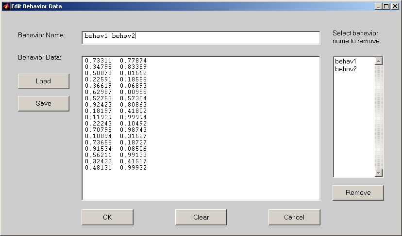
Figure 21

In this window, you can either input behavior data values directly into Behavior Data text editor, or you can click Load button to load a behavior data text file. Once the behavior data is inputted or loaded, you can change the Behavior name to some meaningful string, such as RT and ACC etc. Click OK button when finish. If you deselect any condition after loading behavior data, you have to click Load behavior data button again. This is because the behavior data should correspond to the selected conditions only.

If Mean-Centering Type or Correlation Mode pull-down menu is enabled, you can have the opportunities to choose different values. If you do not know how to do so, please leave the default value (i.e. 0) unchanged, so the conventional mean-centering or correlation algorithm will be applied. The meanings of these two menus are provided by N. Kovacevic below.

Mean-Centering Type feature allows you to choose the kind of mean-centering of the data matrix before running Mean-Centering Task PLS, Non-Rotated Task PLS, Multiblock PLS, Non-Rotated Multiblock PLS. Depending on your scientific question, by selecting a specific type for mean-centering you can remove main effects that are not of interest and focus on those that are relevant. The options are as follows:

0 - (default) Within each group remove group means from conditon means. Tells us how conditions are modulated by group membership. Boosts condition differences, removes overall group differences. Best suited if you are interested in condition and condition- by-group effects.

1 - Remove grand condition means from each group condition mean. Tells us how conditions are modulated by group membership. Boosts group differences, removes overall condition differences. Best suited if you are interested in group and group-by-condition effects.

2 - Remove grand mean (over all subjects and conditions). Tells us full spectrum of condition and group effects (group, conditions and group-by-condition).

3 - Remove all main effects, subtract condition and group means (group by condition). This type of analysis will deal with pure group by condition interaction.

Correlation Mode feature applies to Regular Behav PLS, Non-Rotated Behav PLS, Multiblock PLS, Non-Rotated Multiblock PLS. You can choose among different measures of association between brain data and behavioral data. The options are as follows:

0 - (default) Pearson correlation

2 - Covaraince

4 - Cosine angle

6 - Dot product

Permuatation tests are used for significance testing, where an effect size, measured by the corresponding singular value is tested for being grater than chance using permutations. In order to run Permutation tests, you need to set values greater than 0 for Number of Permutation loops.

Within each Permutation loop, you can also run additional Number of Split loops for reliability tests. The Splithalf resampling examines each latent variable for the reliability of association between brain and design patterns. If you want to learn more about the Splithalf resampling, please read the paper in the link: http://www.utdallas.edu/~herve/abdi2013-kabam-plscv.pdf. In this case, PLS application will estimate two p-values, which reflect the reliability of the brain pattern (p_ucorr) and the design pattern (p_vcorr). Simulations have shown that this type of testing is less prone to false positives and may improve detection rate. However, this option is computationally more demanding. In order to run Splithalf resampling, you need to set values greater than 0 to both Number of Permutation and Number of Split fields. Good rule of thumb is to choose 100 for both values. If you have parallel computing toolbox for Matlab, it is a good idea to set matlabpool open, because it will considerably speed up the tests. If your computer is not fast enough to run Splithalf permutation, you can disable this option by setting Number of Split field to default value (i.e. 0).

Reliability of individual voxels, as part of a brain pattern is tested using Bootstrap resampling. In order to run Bootstrap tests, you need to set values greater than 0 for Number of Bootstrap loops. However, make sure you have enough subjects, because we reorder bootstrap data with replacement and it contains repeated subjects after reordering. The bootstrap result includes the upper and lower percentile of Correlations or Brain Scores. It is determined by the value in Confidence Level field, which is 95 percent by default.

The Bootstrap resampling for Splithalf permutation is different from the conventional one, because the conventional one includes the procrustes rotation. Simulation shows that use of the procrustes rotation has a significant effect on p-value, but very little effect on bootstrap results. Therefore, no procrustes rotation is applied during Bootstrap resampling for Splithalf permutation, and single p-value associated with a singular value is equivalent to the Non-Rotated PLS method.

You can either click Run button to run PLS analysis right away, or click Save to Batch button to save the PLS analysis setting into a batch file. In either case, you will need to input a result file name first. The saved batch file can be used in Batch Process to get the result file in batch. It can also be used to save your PLS analysis setting, and you can bring the setting up in the future by clicking Load from Batch button and select this saved batch file.

7. Show PLS Result

This User's Guide only describes how to display a PLS result file. If you would like to know how to interpret your result, please refer to relevant papers.

7.1. Displaying PET result file

In the PLS start window, click PET button and the button will be highlighted. Then click Show PLS Result for PET data button below, you will be asked to select a result file. Once you have selected the result file, the PET Result window will open (Figure 22). All slices are displayed, and slice indices are equal to X value plus Y value. This kind of labeling is very helpful in zooming.

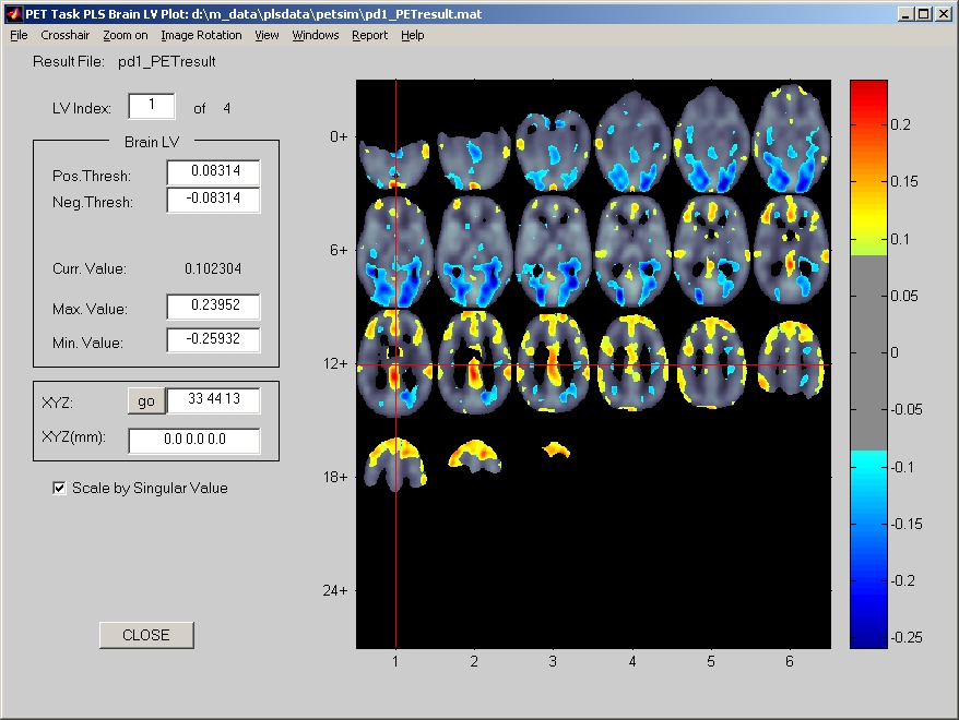
Figure 22

If the result file contains a bootstrap result, the result window will display a view of Bootstrap Ratio first, and you can switch to a view of Brain LV by clicking View menu. Otherwise, the result window will display a view of Brain LV, and there will be no View menu.

Image Rotation menu provided limited amount of rotations for display only. If you want to change image orientation, you have to do so in Creating PET sessiondata file step.

If the crosshair bothers you, you can turn it off or change its color under Crosshair menu. You can click Zoom on menu to get a closer look at the region of interest.

Here we use two different thresholds (Pos / Neg Thresh) just in case the distribution of data is extremely biased. Therefore, it is still suggested to use symmetric threshold, and it is not recommended to modify the threshold arbitrarily, unless you know what you are doing.

Most information in result data is rendered under Windows menu.

7.1.1. Singular Values Plot

Singular values are usually checked first (Figure 23).

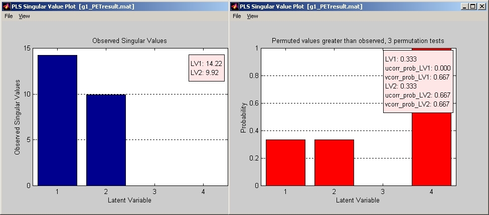
Figure 23

Click Singular Values Plot under Windows menu, and the Singular Value Plot window will open (blue bar). If the value is very low for certain LVs, you may want to discard those LVs. If permutation test is included, you can also check whether those LVs are trustable by plotting the permuted singular value. Click Permuted Singular Values under View menu of Singular Value Plot window, Permuted Singular Plot window will open (red bar). It is the probability of those permuted singular values that are greater than the observed singular values. If the chances that permuted singular values are greater than the observed singular values are very high for certain LVs, you may also want to discard those LVs.

7.1.2. Voxel Intensity Response

To view voxel values in the created datamat, click Voxel Intensity Response under Windows menu, and the response window will open behind the result window. If you click anywhere of the brain in result window, voxel value in the location that is specified by XYZ will be plotted (Figure 24).

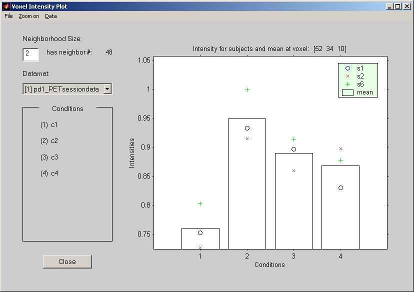
Figure 24

Different subjects can be distinguished by legend mark. Subject average for each condition is provided in bar graph. If you have more than one datamat, select the datamat that you would like to watch from the Datamat selection box.

You can use average intensity of the neighborhood voxels for intensity of the clicked voxel by specifying Neighborhood Size field (An edit box in Voxel Intensity Plot window). By default, it is 0, which means no neighborhood voxel is included. Otherwise, neighborhood size represents the distance (number of voxels) from the clicked voxel. In this case, the average intensity will include those voxels:

The clicked voxel.
The stabled voxels that meet the bootstrap threshold criteria, if bootstrap result is available.
The clustered voxels of the current view. (Cluster mask of BrainLV View is different from that of Bootstrap View).

Do not set neighborhood size unnecessary large, because the maximum number of neighborhood voxels is equal to the cubic of� (SIZE * 2 + 1). e.g. Neighborhood Size 1 could have a neighborhood of 27, and Neighborhood Size 3 could have a neighborhood of 343, etc.

7.1.3. Multiple Voxels Extraction

To extract voxel values from created datamats to a text file, you should prepare a voxel location text file in advance. This file contains XYZmm positions. It must be voxel location with unit in millimeter, instead of absolute voxel location XYZ. One row stands for each voxel, XYZmm are separated by spaces, like:

�� 32.0 24.0 -20.0

�� -36.0 -48.0 -4.0

Click Multiple Voxels Extraction under Windows menu, and select the above voxel location file. Input only a prefix of the extracted file name, and you will be prompted to select a voxel neighborhood size to use average intensity of the neighborhood voxels for intensity of the selected voxels in your location file. It works the same way as the neighborhood voxels we discussed above. Click OK button, it will generate two kinds of files:

prefix_MODULEvoxeldata.txt:� This file includes all subjects in all groups. The rows of this file are in the order of subjects in conditions in groups.
prefix_MODULE_grp_[subj]_voxeldata.txt:� Each of these files will correspond to each session/datamat pair.

Columns of the extracted files stand for voxels in the order listed in the voxel location file. For E.R.fMRI, each voxel will take multiple columns which stand for multiple lags (the size of temporal window).

7.1.4. Design LV and Design Scores Plot

For Mean-Centering PLS, Non-Rotated Task PLS, or Multiblock PLS, you have the option to click Design LV and Design Scores Plot under Windows menu, and the plot window will open (Figure 25).

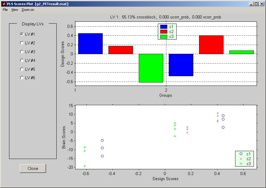
Figure 25

This window has three views: Brain Scores vs. Design Scores, Design Scores and Design LVs. Click View menu in this window to switch between views. If the result has more than one LV, select the LV that you would like to watch in the left panel. Usually the first thing you may want to check is the outlier subject(s) in the Brain Scores vs. Design Scores view. If there are any outlier subjects, you may want to reconsider whether you want to keep them or remove them. If you decide to remove them, you will have to run analysis again without those subjects.

7.1.5. Task PLS Brain Scores with CI

For Mean-Centering PLS and Non-Rotated Task PLS, you also have the option to click Task PLS Brain Scores with CI under Windows menu, and the plot window will open (Figure 26).

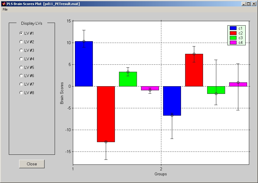
Figure 26

For Behavior PLS or Multiblock PLS, the following submenu will also be available under Windows menu: Brain Scores vs. Behavior Data Plot, Datamat Correlations Response, and Datamat Correlations Plot.

7.1.6. Brain Scores vs. Behavior Data Plot

Click Brain Scores vs. Behavior Data Plot submenu will start with the Brain Scores Plot window (Figure 27).

Figure 27

It displays brain scores vs. behavior data for each condition and each LV. If you have more than one group, select the group that you would like to watch in the upper left panel. If the result has more than one LV, select the LV that you would like to watch in the lower left panel. The title of each plot shows which LV is currently selected, and the variable r stands for correlation coefficient between behavior data and datamat.

You can click Show Brain Scores Overview under Plot menu to view all plots of different conditions and behavior measures (Figure 28).

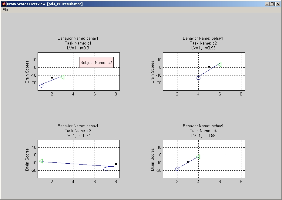
Figure 28

Click Show Correlation Plot under Plot menu will display the correlation bar. It reflects the correlations between behavior data and brain scores. If bootstrap test is included, correlation bar will come with an error bar specified by upper and lower error range for the correlation. You can also select different groups and LVs in the same way above. Click Show Correlation Overview under Plot menu to view a correlation bar that includes all groups and conditions with all behavior measures (Figure 29).

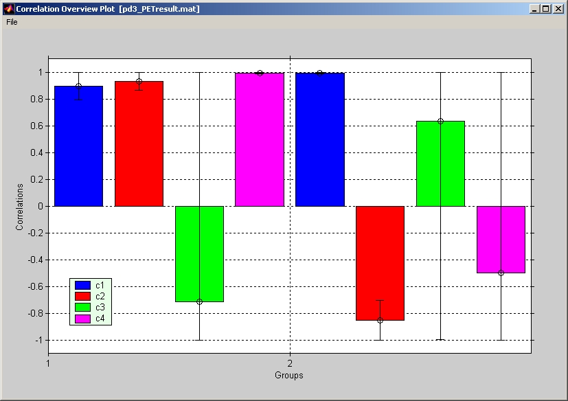
Figure 29

Click Show Behavior LV Overview under Plot menu to view Behavior LV bar for all groups and conditions (Figure 30).

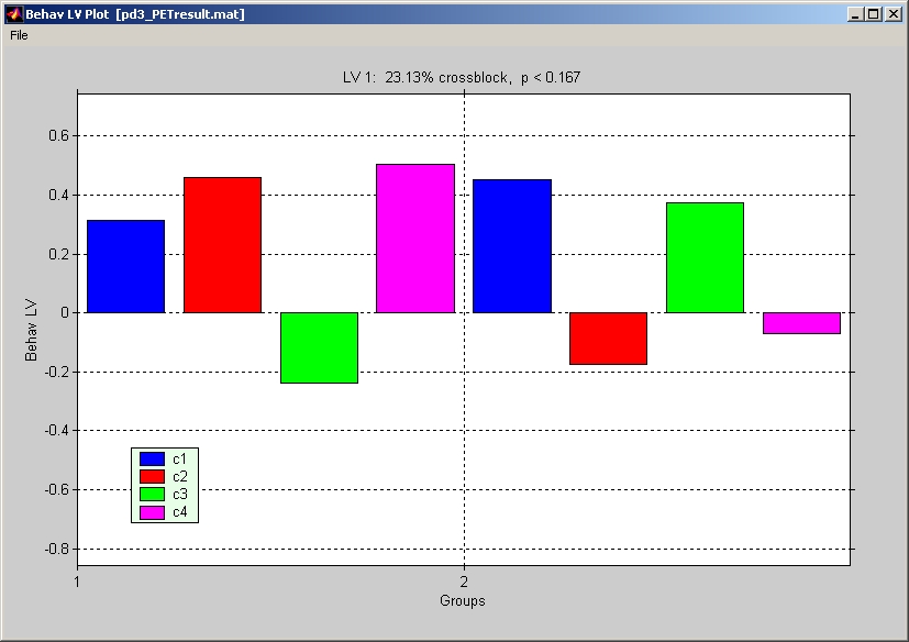
Figure 30

7.1.7. Datamat Correlations Response

The Datamat correlations are correlation between behavior data and datamats. Click Datamat Correlations Response under Windows menu, and the response window will open behind the result window. If you click anywhere of the brain in result window, correlation value at XYZ will be plotted in bar graph (Figure 31).

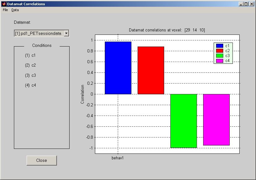
Figure 31

7.1.8. Datamat Correlations Plot

Like datamat correlations in the above response window, Datamat Correlations Plot window also reflects the correlations between behavior data and datamats. However, Datamat Correlations Plot gives you an overview of the correlation values in the entire brain for each condition and each behavior measure (Figure 32).

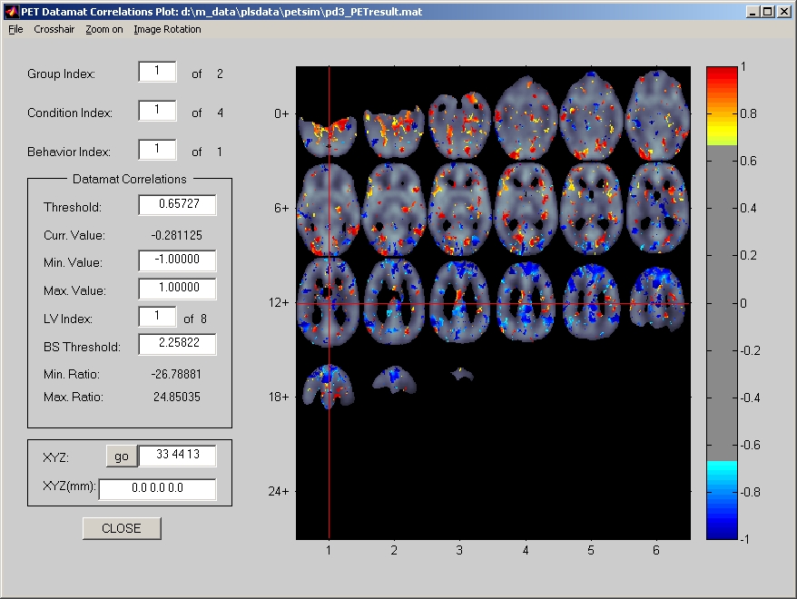
Figure 32

Instead of selecting a group name from selection box, you need to enter a group ID, which is ordered sequentially, in Group Index field. Parameters in Datamat Correlations frame below that are merely for display purposes. Only those voxels with values that are above the Threshold (and BS Threshold if bootstrap test is included) will be displayed. Voxel's datamat correlation value is referred by to its color.

7.1.9. Cluster Report

We define it as a cluster if there are at lease N voxels connected together (5 voxels by default), and we call the one with the highest value as peak voxel. If the distance between the peak voxels of any two clusters is too close (10 mm by default), they will be treated as one cluster. Report menu provides you with capabilities of creating and loading a cluster report. You can also click Set Cluster Report Options under Report menu to change the default setting. Don't change Origin location field unless you have a good reason.

The accuracy of cluster report also depends on the recursion limitation of the MATLAB on your computer. Because of this recursion limit, you may encounter active voxels in the same cluster are separated into two or more clusters, some active cluster are not listed, the result of cluster report are different from one computer (or MATLAB version) to the other. Please refer to the FAQ.txt for more details.

Click Create Cluster Report under Report menu will generate cluster report for the current view (either Brain LV or Bootstrap). The report will display Voxel Mean, XYZ (absolute location), XYZ in mm, Brain LV Value or Bootstrap Value, and Cluster Size in voxels for the peak voxels of all clusters that are listed sequentially. It will also display the Source result file name, Current LV index, Current Threshold, Minimum Cluster Size, and Minimum Cluster Distance at the bottom (Figure 33).

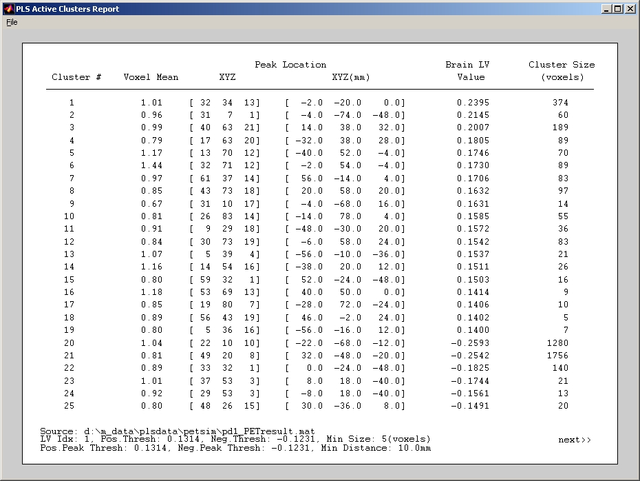
Figure 33

There are two Save submenus and two Export submenus under File menu of Cluster Report window.

Save to .mat file saves cluster_info structure into a MATLAB file, which can be loaded from Load Cluster Report under Report menu.
Save to .txt file writes the content on Cluster Report window to a plain text file.
Export All Locations writes XYZmm locations of all cluster voxels to a plain text file.
Export Peak Location writes XYZmm locations of only peak voxels to a plain text file.

Select Cluster Mask under Report menu to display only the clustered voxels. However, you must create or load cluster report first. Then you can either close the cluster report window or leave it on.

7.1.10. File menu

If you would like to view a brain template underlying the result plot, you can click Load Background Image under File menu and select the brain template image as background image. The background image must have the same dimension as the images that are used in datamats.

Save brain region to IMG file takes the coordinates of the common brain region from the result file, and saves it to a brain region image file.

Save Current Display to IMG files saves the result image that is currently displayed to image files, and it also saves the colormap of current figure to a MATLAB file that is ended with "_cmap.mat".

Save the BLV (or BSR) result to IMG files saves the result values (either Brain LV or Bootstrap Ratio) that are currently displayed to image files.

7.2. Displaying Structural MRI result file

The way to display a Structural MRI result file is the same as the way to display a PET result file.

7.3. Displaying Blocked fMRI result file

The way to display a Blocked fMRI result file is the same as the way to display a PET result file.

7.4. Displaying E.R.fMRI result file

The way to display an E.R.fMRI result file is a little bit different from the way to display a PET or a Blocked fMRI result file. Here are the differences:

7.4.1. Different slices layout in result window

E.R.fMRI displays all lags of temporal window in the result window (Figure 34).

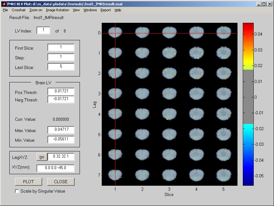
Figure 34

Lag stands for scan in temporal window, which starts from 0. Lag is displayed on Y-axis, and each row displays all the slices that are selected. This is very different from Blocked fMRI or PET display, which do not have lag information. In Blocked fMRI and PET result widnow, all slices are displayed row by row.

Slices are selected from the left panel. When you specify a First Slice index, a Step, and a Last Slice index. It will display the first slice, and slices for every step. If any slices go beyond the last slice, they will not be displayed. When you select a voxel from LagXYZ field instead of clicking on the brain, please make sure that the slice index you entered is currently displayed. Otherwise, it will prompt warning that Invalid number in X, Y, or Z.

7.4.2. Response Function Plot vs. Voxel Intensity Response

Response Function Plot window in E.R.fMRI plots the intensity change of a clicked voxel for the entire temporal window. Its counterpart in Blocked fMRI and PET is Voxel Intensity Response window, which does not have temporal window time series information.

In Response Function Plot window (Figure 35), all subjects for each condition take one row, with an average plotted at the end. Intensity value is displayed on Y-axis, and Lag number is displayed on X-axis. If bootstrap test is included, special symbols (small circle and diamond) will also be marked at top and bottom of each plot to represent the stable time points for the 1st & 2nd LVs. Click Stable off menu to hide those stable symbols.

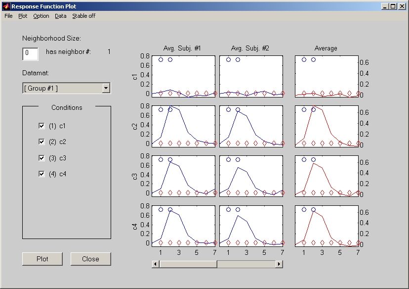
Figure 35

There is an Export Data under Data menu of the response window. The row order of st_data variable in the exported data is determined by st_evt_list variable. However, we suggest people to use Multiple Voxels Extraction under Windows menu. This way, you can get all voxels' data at once. In addition, you do not have to worry about the order of rows, which is always in the order of subjects in conditions in groups.

You can change the display appearance by selecting submenus under Option menu. For example, to Hide / Show Average Plot; to Combine / Separate plots within conditions; to Enable / Disable Data Normalization; etc.

7.4.3. Temporal Brain Scores Plot

For Mean-Centering PLS, Non-Rotated Task PLS, or Multiblock PLS, there is a submenu under Windows menu for E.R.fMRI result. It is called Temporal Brain Scores Plot, and displays the brain scores for the entire temporal window. The appearance and usage of Temporal Brain Scores Plot window is very similar to Response Function Plot window. However, it opens in front of the result window. You need to click Plot button to display, and click LV radio button to select which LV you would like to watch.

7.4.4. Temporal Brain Correlation Plot

For Behavior PLS or Multiblock PLS, there is a submenu under Windows menu for E.R.fMRI result. It is called Temporal Brain Correlation Plot, and displays the correlations between behavior data and brain scores for the entire temporal window. Since brain scores in result file do not contain time series information, we have to generate it from a subset of Datamats and Brain LV on fly for each lag of temporal window. The appearance and usage of Temporal Brain Correlation Plot window is very similar to the Temporal Brain Scores Plot window, and both windows open in front of the result window.

7.4.5. Different Datamat Correlations Response window

Datamat Correlations Response window in E.R.fMRI plots the correlations between behavior data and datamats of a clicked voxel for the entire temporal window. Its counterpart in Blocked fMRI and PET does not have time series information. The appearance and usage of Datamat Correlations Response window is very similar to the Temporal Brain Correlation Plot window. However, it opens behind the result window. If you click anywhere of the brain in result window, correlation value for the entire temporal window at XYZ will be plotted.

7.5. Displaying ERP result file

The way to display ERP result file is much different from the way to display Blocked fMRI, E.R.fMRI, or PET result file.

In PLS start window, click ERP button and it will be highlighted. Then click Show PLS Result for ERP data button below, you will be asked to select a result file. Once you select the result file, ERP Electrode Salience waveform window will open (Figure 36). It plots the salience on each electrode, and uses menu to control the display. If you click any waveform, a pink information box that contains channel name and wave name will be popped up.

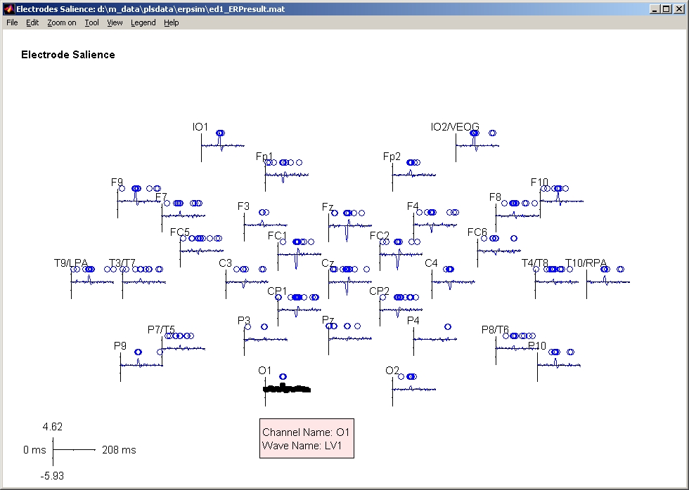
Figure 36

7.5.1. TOOL menu

Under Tool menu, there is a Display Options submenu. If bootstrap test is included, there is also a Bootstrap Options submenu.

In Display Options window, you can select which waveform(s) to be displayed. If you click Select All Waves button, all waves will be displayed. However, the more waves you selected, the longer it will take to display. You can also change axis intervals and font size by selecting the proper values beside them. If electrodes are distributed too sparse (or too crowded), you can also adjust the Wave Size scroll bar to change the wave size for every electrode.

Bootstrap stability is displayed in small circles or diamond. A circle will be marked at the time point that the bootstrap value exceeds the threshold. Bootstrap from different LV will take different horizontal lines. In Bootstrap Options window, there are 2 panels. The left panel displays the LV to be edited. You can only select 1 LV at a time to edit it. The parameters below that panel (Threshold etc.) can be edited and are all for the LV that you selected in the left panel. Click Reset to default value will reset those parameters to their default values. The right panel displays the LV to be displayed in Electrode Salience window. You can select one or more LVs to be displayed at the same time.

7.5.2. LEGEND menu

Click Legend On under Legend menu to display color legend for the wave and bootstrap displayed in the waveform window. Click Legend Off will remove the color legend. Because the limitation of MATLAB, it will be very slow if this is your first click of Legend On. Especially when there are a lot of waveforms displayed. After you click Legend Off, the subsequent clicks of Legend On will be quick.

7.5.3. ZOOM menu

Click Zoom on to have a closer look at a few electrodes. Click Zoom off to cancel the zooming status. Actually, we have another way to do it using Plot Detail under the View menu.

7.5.4. EDIT menu

There are 3 submenus under Edit menu. They are: Select Electrodes with Rubberband, Select All Electrodes, and De-Select All Electrodes. As is known by the submenu names, they are used to select or deselect electrodes. The other way to select an electrode is to click the electrode name directly and make it bold. After an electrode is selected, its detail can be plotted using Plot Detail under View menu.

The reason that we call this menu Edit is because we can visually screen out bad subjects and/or electrodes in ERP Amplitude window immediately after creating or modifying ERP sessiondata file. In ERP Amplitude window, you can select a bad subject by selecting the bad subject waveform, and select a bad electrode by clicking its names and making it bold. Then click Modify Datamat under Edit menu, the Modify Datamat window opens, and the selected subjects and electrodes are preliminary un-highlighted. Once you click Modify button in Modify Datamat window, the bad subjects and electrodes will be removed from the sessiondata file.

7.5.5. VIEW menu

This is the main menu to get information from the result data. There are several submenus under View menu, they are: Subject Amplitude, Average Amplitude, Spatiotemporal Correlation (only for Behavior PLS and Multiblock PLS), Plot Detail, Plot Singular Values, Plot Design Scores (not for Behavior PLS), Plot Temporal Scores (not for Behavior PLS), Plot Scalp Scores (only for Behavior PLS and Multiblock PLS), Plot Temporal Correlation (only for Behavior PLS and Multiblock PLS).

Subject Amplitude

Click Subject Amplitude under View menu will open Group Subject Amplitude waveform window. It plots the ERP amplitude of all subjects in all conditions and all groups that are used by this result.

Like Electrode Salience window, you can open Display Options window under Tool menu to select which waveform(s) to plot. However, this Display Options window is different from that from Electrode Salience window. In this Display Options window, you can easily select all subjects in a certain condition or all conditions in a certain subject by selecting the proper pull down menu.

Average Amplitude

Click Average Amplitude under View menu will open Grand Average Amplitude waveform window. It plots the average ERP amplitude of all subjects in a particular condition and a particular group.

It also has its own Display Options window under Tool menu to select which one to plot. If bootstrap test is included, you can also open Bootstrap Options window, and the Bootstrap Options window is exactly like what you see in the Electrode Salience window.

Under Tool menu of Grand Average Amplitude window, there are 2 more submenus: Display Condition Average and Display Condition Difference.

Display Condition Average allows you to display the average of the existing average waves. You can select several conditions from the left panel, give a name for the newly averaged condition, and click ->> button to make the averaged condition. The default averaged condition name will be the one with plus signs inserted among selected conditions.

For Display Condition Difference, it allows you to display the waveform of one condition subtracted by the other. Once you open the Condition Difference window, click Add button first. Then, select two conditions from the pull down menu.

Spatiotemporal Correlation

If it is a result of Behavior or Multiblock PLS, you can click Spatiotemporal Correlation under View menu to display the correlation waveform between behavior data and datamats. The usage is very similar to the Subject Amplitude waveform window, and its counterpart in other modules is called Datamat Correlation Plot.

Plot Detail

If you only want to plot some of those electrodes, you can open Plot Detail window once you have selected one or more electrodes. You know the electrodes are selected if their names become bold. Click on the names can toggle the electrode select or deselect. You can also select or deselect electrodes using the tools provided under Edit Menu.

In Plot Detail window (Figure 37), it only displays the waveforms of the selected electrodes, with detail grid and units. If you click on any waveform, an pink information box that contains wave name, channel name, X & Y locations will be popped up.

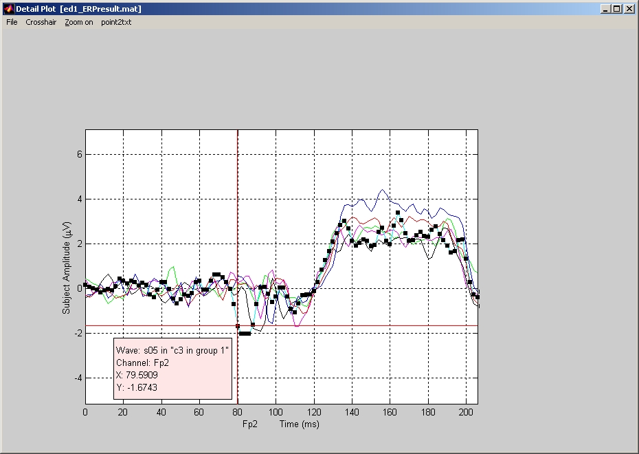
Figure 37

Subject Amplitude for Given Timepoints

It looks like Plot Detail window with two more menus: Response Plot and Multiple Extraction, and you can plot the response of datamat value and extract multiple time points from this window.

To plot the response, click Response Plot menu in this window, and the Response Plot window will pop up and then stay behind the current window. The Response Plot window looks exactly the same as the Voxel Intensity Response window in PET.

To extract multiple time points, you need to prepare a time points file in advance. The time points file contains a single column of data, and each row represents a time point in milliseconds. When you click the Multiple Extraction menu, you will be prompted for this file. The behavior is the same as its counterparts in all other modules.

Other Submenus

The rest of submenus under View menu are very similar to the ones under Windows menu in E.R.fMRI module. For example, Plot Singular Values is equivalent to Singular Values Plot; Plot Design Scores is equivalent to Design LV and Design Scores Plot; Task PLS Scalp Scores with CI is equivalent to Task PLS Brain Scores with CI; Plot Temporal Scores is equivalent to Temporal Brain Scores Plot; Plot Scalp Scores is equivalent to Brain Scores vs. Behavior Data Plot; Plot Temporal Correlation is equivalent to Temporal Brain Correlation Plot.

8. Seed PLS Analysis

We can use correlation between datamat value from a seed voxel and entire brain datamat to run Regular Behav PLS analysis, and we call this Seed PLS analysis.

8.1. Step-by-Step Procedures

Open a PET, E.R.fMRI or Blocked fMRI result file to the result window, and search for seed voxels.
Write down their XYZmm locations (must be voxel location with unit in millimeter, not absolute voxel location). In order to avoid out of memory problem, please choose only a few positions. For E.R.fMRI, don't worry about lags, since all lags in temporal window will be extracted.
Click Multiple Voxel Extraction under Windows menu to extract multiple voxels for above locations, and it will generate two kinds of files below. However, we only use Format A file here, which includes all subjects in all groups:

Format A:�� PREFIX_MODULEvoxeldata.txt (only 1 file)

�� (This one includes all subjects in all groups)

Format B:�� PREFIX_MODULE_grp_[subj]_voxeldata.txt

�� (Each of these files will correspond to each sessiondata file)

Check the extracted values. If it is all the same for certain column, please remove the entire column. For example, for E.R.fMRI, the baseline lag (lag0) usually contains all 0, and it should be removed.
Start Run PLS Analysis window. Add the same datamats and select the same conditions as you did to create the above result file.
Choose Regular Behav PLS option. Click Load behavior data button, and load the behavior data in format A (including all subjects in all groups). If there is any column (specified by Behavior Name) containing the same Behavior Data value across all rows in the edit window, that column should be removed.
Enter the number of Permutation / Bootstrap (optional), and click Run to run Seed PLS Analysis.

9. Batch Process

Instead of using mouse click, messages can also be loaded from a batch file and sent automatically to GUI interface in batch. The first advantage of the batch process is that it dramatically reduces the Human-Computer Interactions. So, you can issue batches at the end of a day, and the computer will create all the sessiondata files one by one and run all the analysis for you. When you come back next day, a PLS result file is ready for you to display. The second advantage is that it is very easy to modify a batch file to re-create a sessiondata file or re-run an analysis. The third advantage is that the sessiondata files and result files that are generated from batch files are fully compatible with those that are generated from GUI interface. The only disadvantage is that batch files must be checked carefully, especially when you want to run batch overnight.

9.1. How to write a batch file

In order to create datamats or run analyses in batch, you will first need to prepare corresponding batch files. Batch files are simply text files, and we will discuss them in detail in the following sections.

Coming with PLS Applications, you will find several demo batch files:

�� batch_demo_fmri_data1.txt�� % batch file to create E.R.fMRI sessiondata

�� batch_demo_fmri_data2.txt�� % batch file to create E.R.fMRI sessiondata

�� batch_demo_fmri_data3.txt�� % batch file to create E.R.fMRI sessiondata

batch_demo_fmri_analysis.txt�� % batch file to run E.R.fMRI PLS analysis

�� batch_demo_bfm_data1.txt�� % batch file to create Blocked fMRI sessiondata

�� batch_demo_bfm_data2.txt�� % batch file to create Blocked fMRI sessiondata

�� batch_demo_bfm_data3.txt�� % batch file to create Blocked fMRI sessiondata

batch_demo_bfm_analysis.txt�� % batch file to run Blocked fMRI PLS analysis

�� batch_demo_erp_data1.txt�� % batch file to create ERP sessiondata

�� batch_demo_erp_data2.txt�� % batch file to create ERP sessiondata

batch_demo_erp_analysis.txt�� % batch file to run ERP PLS analysis

�� batch_demo_pet_data1.txt�� % batch file to create PET sessiondata

�� batch_demo_pet_data2.txt�� % batch file to create PET sessiondata

batch_demo_pet_analysis.txt�� % batch file to run PET PLS analysis

�� batch_demo_struct_data1.txt�� % batch file to create Structural sessiondata

�� batch_demo_struct_data2.txt�� % batch file to create Structural sessiondata

batch_demo_struct_analysis.txt�� % batch file to run Structural PLS analysis

Once you follow the instructions discussed in the following sections and create your own batch file, you can run them using batch_plsgui command.

You can run several batch files with one batch call. The following command will create an ERP sessiondata file, and run ERP analysis with the created sessiondata file:

batch_plsgui batch_demo_erp_data1.txt batch_demo_erp_analysis.txt

You can also streamline the batch processing by putting multiple batch calls in one M file. The following will create three fMRI sessiondata files, and run fMRI analysis with the created sessiondata files:

batch_plsgui batch_demo_fmri_data1.txt

batch_plsgui batch_demo_fmri_data2.txt

batch_plsgui batch_demo_fmri_data3.txt

batch_plsgui batch_demo_fmri_analysis.txt

The easiest way to get started is to copy a demo batch file that comes with PLS Applications, and then modify it based on your scenario:

Go to plsgui folder in PLS Applications. If you don't know where it is, you can type which plsgui in MATLAB command window to locate the path.
Search batch_demo_MODULE* for MODULE related batch files. e.g. batch_demo_erp* is for ERP related batch files. batch_demo_erp_data1.txt is for creating ERP sessiondata file for group1; batch_demo_erp_analysis.txt is for running ERP analysis.
Copy all related batch files to your working folder that you prepare to keep the result. You may remember that result file must be kept in the same folder as sessiondata files and batch files that are used when creating the result.
Rename the demo batch files, and edit them with the necessary changes. Sections below and comments in those batch files explain how to edit them.
Each batch file is composed of several lines. Empty line or any line starting with "%" will not be parsed. Each line starts with a keyword string (e.g. prefix, num_boot etc.). These keywords should never be changed. Following the keyword is its corresponding value. You can use either tab or space to separate "keyword / value" and "value1 / value2". At the end of value, you also have the option to append a comment starting with "%" character.
Once you have modified (or created) batch files, you can put all batch calls into an M file, so they can be executed one after the other (see batch_demo_*.m).

Tips: The easiest way to get batch file for running PLS analysis is to click Save to Batch button in PLS analysis window. The GUI will automatically write all parameters on PLS Analysis window to a batch file.

9.2. Batch file to create E.R.fMRI sessiondata

Instead of filling the fields in the Session Information window manually, we can put them as the values of keywords in a batch file (see batch_demo_fmri_data1.txt):

Value of prefix keyword is a string (e.g. demo) that will compose sessiondata file name (e.g. demo_fMRIsessiondata.mat).
Value of brain_region keyword can be either a threshold number or a file name with path info that indicates the brain region binary file.
Value of win_size keyword indicates the number of scans in one hemodynamic period.
Value of across_run keyword can be either 1 or 0. Use 1 for merging data across all run for each condition, and use 0 for merging data within each run and then stacked together run by run.
Value of single_subj keyword refers to a feature that does not average all onsets in a condition. To use this feature, set it to 1, and scans that are led by each onset will be treated as an individual block in the datamat. Otherwise, scans for all the onsets will be averaged together as one block.
Value of single_ref_scan keyword refers to a feature that will replace the ref_scan_onset keyword and num_ref_scan keyword below. To use this feature, set it to 1, and all scans in this datamat will use this reference scan.
Value of single_ref_onset keyword is the onset for single_ref_scan keyword above, and starting from 0.
Value of single_ref_number keyword is the number of onset for single_ref_scan keyword above, and starting from 1.
Value of the first cond_name keyword is name of condition1, and the name of condition2 is listed after condition1 in sequence for value of the second cond_name keyword.
Value of the first ref_scan_onset keyword is the reference scan onset for condition1, and the one for condition2 is listed afterwards in sequence for value of the second ref_scan_onset keyword.
Value of the first num_ref_scan keyword is the number of reference scans for condition1, and the one for condition2 is listed afterwards in sequence for value of the second num_ref_scan keyword.
You can re-organize them to let cond_name, ref_scan_onset, and num_ref_scan be grouped together (see batch_fmri_data1.txt). However, sequence should not be changed (i.e. name for condition2 can not be listed before name for condition1). The same rule is also applied to ref_scan_onset & num_ref_scan in condition section and data_files & event_onsets in run section.
Value of the first data_files keyword stands for all selected file names of scan images in run1 with path information. All selected image file names in the run folder should be sorted in alphabetic ascend order that represent scans of this run in time series sequence. Wildcard must be used for all selected file names. Run2 is listed after run1 in sequence for value of the second data_files keyword.
Values of the first event_onsets keyword stand for the onset scans (start from 0) of condition1 in run1. Then, condition2 in run1 for values of the second event_onsets keyword ... etc. So the sequence should always be condition in run.

9.3. Batch file to run E.R.fMRI analysis

As I mentioned above, the easiest way to get batch file for running PLS analysis is to click Save to Batch button in PLS Analysis window. However, if you want, you can also manually create such a batch file (see batch_ demo_fmri_analysis.txt):

Value of result_file keyword is a string for result file name with path information. It must be listed first in the analysis batch file.
Values of the first group_files keyword stand for all sessiondata file names for group1. (In E.R.fMRI or Blocked fMRI, each group can contain more than one sessiondata file, and each sessiondata file can have more than one run). Group2 is listed after group1 in sequence for value of the second group_files keyword.
You have 6 PLS analysis option. Set value of pls keyword to 1 if you would like to do Mean-Centering PLS; set it to 2 for Non-Rotated Task PLS; set it to 3 for Regular Behav PLS; set it to 4 for Multiblock PLS; set it to 5 for Non-Rotated Behav PLS; set it to 6 for Non-Rotated Multiblock PLS.
Value of mean_type keyword refers to mean-centering type. It can be [0 1 2 3], and default value is 0.
Value of cormode keyword refers to correlation mode. It can be [0 2 4 6], and default value is 0.
Value of num_perm keyword refers to number of permutations.
Value of num_split keyword refers to number of split half permutations.
Value of num_boot keyword refers to number of bootstraps.
Value of boot_type keyword refers to bootstrap type. It can be strat or nonstrat, and default is strat (Please do not change this value).
Value of clim keyword refers to confidence level of bootstrap test for Behavior (or Multiblock) PLS.
Value of save_data keyword can be either 0 or 1. Choose 1 if you would like to save the stacked datamat; choose 0 otherwise.
Leave values of selected_cond keyword commented if you do not deselect any condition. Otherwise, use only 1 or 0 for the value of each condition, where 0 stands for the deselected condition (condition for behavior block in multiblock PLS is not deselected here, and they should be deselected by selected_bcond below).
Leave values of selected_bcond keyword commented if you do not deselect any condition for behavior block in multiblock PLS. Otherwise, use only 1 or 0 for the value of each condition, where 0 stands for the deselected conditions (keyword selected_bcond is only applied to conditions for behavior block in multiblock PLS). In addition, you cannot select any conditions for selected_bcond that were deselected in selected_cond.
Values of the first contrast_data stand for the contrast data of selected condition1 in group1. Then, selected condition2 in group1 for value of the second contrast_data keyword ... etc. So the sequence is selected condition in group. Number of values for each contrast_data row should be the same, and it represents the number of contrasts.
Values of the first behavior_data stand for the behavior data of subject1 of selected_condition1 of run1 of group1. The sequence should always be subject in selected_condition in run in group. Number of values on each behavior_data row should be the same, and it represents the number of behavior measures.

9.4. Batch file to create Blocked fMRI sessiondata

It is very similar to Batch file to create E.R.fMRI sessiondata. Here are some differences:

No win_size keyword for Blocked fMRI.
event_onsets keyword is replaced by block_onsets.
block_length keyword is used after each block_onsets to represents the number of scans for each block.

9.5. Batch file to run Blocked fMRI analysis

It is very similar to Batch file to run E.R.fMRI analysis. The only difference would be that all the file names containing fMRI are now replaced by BfMRI.

9.6. Batch file to create ERP sessiondata

ERP sessiondata file is very different from that of E.R.fMRI or Blocked fMRI, since a lot of EEG/ERP parameters have to be added in:

Value of prefix keyword is a string (e.g. demo) that will compose sessiondata file name (e.g. demp_ERPsessiondata.mat and demo_ERPdata.mat).
Value of prestim keyword stands for the number of milliseconds for prestimulus baseline.
Value of interval keyword stands for the number of milliseconds for digitization interval.
Values of chan_order keyword are indices for electrode channels. The best way to obtain them is run MATLAB command:

[chan_order, system] = erp_select_chan

Value of system_class keyword takes structure variable value system.class that was obtained together with chan_order.
Value of system_type keyword takes structure variable value system.type that was obtained together with chan_order.
If your data are in plain text file, leave binary_vendor keyword commented or put none for its value. Otherwise, fill the value of binary_vendor keyword with the name of binary data vendor. They can be NeuroScan, ANT, and EGI.
If your data are in plain text file, leave binary_endian keyword commented, or put none for its value. Otherwise, fill the value of binary_endian keyword with a proper MATLAB machine format, they can be: ieee-le or l, ieee-be or b, ieee-le.l64 or a, ieee-be.l64 or s, vaxd or d, vaxg or g, cray or c, and native or n.
Value of the first cond_name keyword is name of condition1, and the name of condition2 is listed after condition1 in sequence for value of the second cond_name keyword.
All binary data and most plain text data are laid out in a way that each row represents an electrode channel. However, there are a few plain text data that are laid out in a way that each column represents an electrode channel. In the latter case, set the value of chan_in_col keyword to 1.
Value of the first subj_file keyword stands for ERP data file name with path information for subject 1 in condition 1. Then, subject 2 in condition 1 for value of the second subj_file keyword ... etc. So the sequence should always be subject in condition.

9.7. Batch file to run ERP analysis

It is very similar to Batch file to run E.R.fMRI or Blocked fMRI analysis. Here are the differences:

All file names that contain fMRI or BfMRI are now replaced by ERP.
ERP and PET modules use only one sessiondata file for each group_files keyword, while fMRI and BfMRI can use more sessiondata file names.
The sequences should be subject in selected_condition in group for the value of behavior_data keyword.

9.8. Batch file to create PET sessiondata

It is very similar to Batch file to create ERP sessiondata. Since PET does not use any of EEG/ERP parameters, those keywords can all be removed except prefix, cond_name, and subj_file. However, brain_region and normalize keyword needs to be added in. brain_region value can be either a threshold number or a file name with path information that indicates the brain region binary file. normalize value is either 1 or 0, and keep it as 1 (normalize volume mean) unless you have good reason not to do so.

9.9. Batch file to run PET analysis

It is very similar to Batch file to run ERP analysis. The only difference would be that all the file names containing ERP are now replaced by PET.

9.10. Batch file to create Structural sessiondata

It is very similar to Batch file to create PET sessiondata. Here are the differences:

Since Structural module cannot use threshold, a pre-defined brain region image file must be used for brain_region keyword.
Value of dataset_path keyword is a string that represents subject files' folder.
Value of normalize keyword should be kept as as 0 (do not normalize volume mean) unless you have good reason not to do so.
Value of cond_filter keyword is a string of wildcard to distinguish different conditions.
Value of subj_name keyword is a string of subject's name.
Value of subj_file keyword is just the subject's file name, and does not need to include its path.

9.11. Batch file to run Structural analysis

It is very similar to Batch file to run ERP analysis. The only difference would be that all the file names containing ERP are now replaced by STRUCT.

10. Appendix

10.1. Appendix A: Test Data Sets

The subjects' data below is only for the purpose of illustrating the usage of PLS applications:

http://pls.rotman-baycrest.on.ca/source/Testdata.zip

After unzip the above data, go to the unzipped "Testdata" folder and launch MATLAB from there. Follow the instructions below for the experiments.

10.1.1. PET Experiment

In this experiment, session files were created (in old style: session / datamat file pair), and result file has been generated.

There are 12 subjects with 8 conditions in this experiment. Click Show PLS Result for PET data button, and open the "pet_PETresult.mat" file. The displayed plot is Bootstrap Ratio Plot. Click View Brain LV under View menu to switch to Brain LV Plot.

Click Design LV and Design Scores Plot under Windows menu to open PLS Scores Plot window. As you can see that all "sent" conditions (sent enc, sent r1, sent r2, and sent r3) are positive, and all "pict" conditions are negative for LV1. This means that the red activation areas in Brain LV Plot correspond to sent conditions, while the blue activation areas correspond to pict conditions.

10.1.2. fMRI Experiment

In this experiment, you only have one subject's data. You can follow the steps below to see how to create sessiondata file, and run PLS analysis to generate result file.

This subject performed 2 tasks with 1 baseline condition (Task1, Task2, and Baseline). There are totally 5 runs that are located in 5 sub-folders (from dataset_001 to dataset_005). Each run lasts 6 minutes with TR of 2 seconds. So this gives us 180 time points (in TR) starting from 0, and each time point is represented by a scan image.

The onsets time points (in TR) of Task1 appeared at: 0 24 48 72 96 120 144 168

The onsets time points (in TR) of Task2 appeared at: 12 36 60 84 108 132 156

The onsets time points (in TR) of Baseline appeared at: 6 30 54 78 102 126 150

In this experiment, all images have been properly spatially and temporally realigned, normalized, and smoothed. In addition, only 5 slices from the entire brain were used. The first step of the experiment is to create a sessiondata file:

Click E.R.fMRI button in PLS start window, and click Session Profile for fMRI data button, the fMRI session window will open.
Type test in Datamat Prefix field.
Leave Across All Runs for Merge Data field.
Click Edit Conditions button, and Edit Condition window will open.
Type Task1 for condition1 field under Condition Name column, and click Add button.
When condition2 field shows up, type Task2 for condition2 and click Add button.
For condition3, type in Baseline and click Add button.
Now, click DONE button to close the Edit Condition window, and you will find the value in Number of Conditions field becomes 3.
Type 5 in Number of Runs field, and click Edit Runs button beside it, a Run Information window will open.
Type 180 in Number of Scans field.
Leave 0 for Number of Scans to be skipped field.
Click Browse button to open Select Data Files window.
Click dataset_001 in the Directories panel and click Select All button.
Click DONE button to close the Select Data Files window.
Click Load Onsets from a text file under Edit menu, and select onsets.txt file.
Keep Replicate trial information across run check box selected. This means that the onset values will be the same across all runs.
Click >> button to proceed to the second run.
You will find that the number 180 is already in Number of Scans field. If the number of scans that selected for your second run is not 180, you need to re-enter the number.
Leave 0 for Number of Scans to be skipped field.
Click Browse button like you did in the first run, and open Select Data Files window.
Click dataset_002 in the Directories panel and click Select All button.
Click DONE button to close the Select Data Files window.
Click >> button to proceed to the next run, and repeat the above steps for all 5 runs.
Click DONE button to close the Run Information window.
Click Create ST Datamat button, and PLS will open a Generate ST Datamat window.
In Generate ST Datamat window, leave everything as default, and click Create button to generate datamat. Once the generating process indicated by a progress bar is finished, you are back to the session window.
Click Close button to close the session window, and you are now in the start window.

You can now run PLS analysis using the above sessiondata file and datamat file. Usually, you should have more than one subject for PLS analysis, and each subject has one sessiondata file. This is especially required for permutation or bootstrap test. Here we only have one subject for illustration purpose, so the following step will run Mean-Centering PLS without permutation or bootstrap test:

Click E.R.fMRI button in PLS start window, and click Run PLS Analysis on fMRI data button, the PLS Analysis window will open.
Click Add button to open Select Session Profile Window.
Highlight test_fMRIsession.mat file name, and click >> button in the middle. Then click DONE to close Select Session Profile Window.
Click Mean-Centering PLS button in PLS option frame.
Leave everything as default, and only click Run button.
Now PLS will prompt you to enter a result file name. You can either select a new result file name, or simply use the default one test_fMRIresult.mat as file name.
Once PLS analysis is done, it goes back to the start window.
In order to view the result data, you need to click E.R.fMRI button in PLS start window, and click Show PLS Result for fMRI data button. PLS will prompt you to select a result file name, and you can select test_fMRIresult.mat to display this result file.

10.2. Appendix B: Command-Line PLS

As is mentioned earlier, the Command-Line PLS pls_analysis is the computation part of PLS Applications. However, its result cannot be displayed with GUI interface, because it is only part of the GUI result.

In order to run pls_analysis, the following input variables must be assigned properly:

datamat_lst: Datamat list cell array. Each cell stands for one datamat (2-D Matrix), which is also referred as a group. All datamats must be in the form of subjects in conditions.
num_subj_lst: Number of subject list array, containing the number of subjects in each group.
num_cond: Number of conditions in datamat_lst.
option: A struct of optional inputs. It can be:

o method: This option will decide which PLS method that the program will use:

1. Mean-Centering Task PLS

2. Non-Rotated Task PLS

3. Regular Behavior PLS

4. Regular Multiblock PLS

5. Regular Multiblock PLS

6. Non-Rotated Multiblock PLS

If it is not specified, program will use default value 1.

o num_perm: If specified and num_perm > 0, PLS will run permutation test with num_perm amount of samples; otherwise, num_perm will use default value 0, and program will not run permutation test.

o is_struct: If it is not specified, is_struct will use default value 0. If specified and is_struct = 1, PLS will not permute conditions within a group. You only need to specify it when you run Non-Behavior Structure PLS and the segmented data is used.

o num_split: If specified and num_split > 0, PLS will run additonal loops for splithalf reliability test; otherwise num_split will take default value 0, and program will not run splithalf.

o num_boot: If specified and num_boot > 0, PLS will run bootstrap test with num_boot amount of samples; otherwise, num_boot will use default value 0, and program will not run bootstrap test.

o clim: Confidence level between 0 and 100. If not specified, program will use default value 95.

o bscan: In Multiblock PLS, you can specify a subset of conditions that are used in multiblock PLS behav block. e.g., bscan=[1 3] for 4 conditions. If it is not specified, it means that all the conditions are selected. Using the above example, bscan is equivalent to [1 2 3 4] for 4 conditions. This option can be applied to method 4 and 6.

o stacked_designdata: If you are choosing Non-Rotated Task PLS, Non-Rotated Behavior PLS, or Non-Rotated Multiblock PLS, you have to specify this 2-D numerical matrix.

o stacked_behavdata: If you are choosing any Behavior PLS or Multiblock PLS, you have to specify this 2-D numerical matrix.

o meancentering_type: Type of meancentering. If it is not specified, program will use default value 0. This option can be applied to method 1, 2, 4, and 6.

o cormode: correaltion mode determines correlation type to analyze. If it is not specified, program will use default value 0. This option can be applied to method 3, 4, 5, and 6.

o boot_type: It can be strat or nonstrat, and default is strat (Please do not change this value).

Once the input variables are prepared, you can run PLS analysis with the following command:

result = pls_analysis(datamat_lst, num_subj_lst, num_cond, [option])

The output result is a structure variable that contains all the necessary items that are generated based on different PLS options. It could have items like:

u: Brainlv or Salience
s: Singular value
v: Designlv or Behavlv
usc: Brainscores or Scalpscores
vsc: Designscores or Behavscores
datamatcorrs_lst: Correlation of behavior data with datamat, only available in behavior PLS
lvcorrs: Correlation of behavior data with usc, only available in behavior PLS
perm_result: struct containing permutation result
perm_splithalf: struct containing permutation splithalf
boot_result: struct containing bootstrap result

Since command-line PLS requires you to provide a datamat cell array, it doesn�t have to be image data or EEG/MEG data that is required by PLS Applications. The following appendix is a tool in plscmd folder that allows people to plot the result of command-line PLS using Region of Interest (ROI) data.

10.3. Appendix C: Plot Bootstrap Results for Region of Interest (ROI) analyses

When you assign data to datamat_lst variable, it can be ROI values. The plotroi tool in plscmd folder to plot bootstrap result of ROI analysis on a template image. The color of each region reflects the corresponding bootstrap ratio (salience/salience standard error). Thresholds as well as minimum and maximum bootstrap ratios are shown on the accompanying color bar.

Before plotting any results, you need to make a flood-filled template image. This image can be created each time you use this tool. However, if you saved this flood-filled image, you can save some steps and load it directly.

Three files are required to run this tool, and optional files (below) make it easier to use.

Required files:

A template image or a flood-filled image:

Template image: The template image should be a gray-scale image in any format that can be read by MATLAB software. Image type and number of bits (e.g, 8 or 16) are not important.� The centre of the ROIs and background should be whiter than the lines used to indicate ROI boundaries. All boundaries must be closed.
Flood-filled image: An image that is created by this tool based on the template image and ROI seed location file (below).

�

An ROI seed location text file:

This file should have the following format:

1�� 252� 263� CBM_Left

2�� 448� 262� CBM_Right

3�� 266� 157� AngularGy_Left

4�� 444� 165� AngularGy_Right

The 1st column is ROI number, and would typically be a vector 1:MaxNumberOfROIs. Use of this module will be most efficient if the order of this file is the same order that you typically use for analysis.

The 2nd and 3rd colums are the x and y coordinates of a seed point location inside each ROI (integer). If your favourite drawing software does not provide this information, you can obtain these coordinates by displaying the image in MATLAB and using the ginput or getpts command to generate the coordinates.

The 4th column is the name of region. If you omit the 4th column, the name of region will be automatically called Region 1, Region 2 etc.

�

A bootstrap ratio text file:

If you obtain the bootstrap data using the command-line PLS, it is actually:

result.boot_result.compare_u

You can save this variable as a text file using this MATLAB command:

save -ascii my_compare.txt result.boot_result.compare_u

�

Optional files:

A text file containg a column vector of ROIs used for the analysis. e.g.:

An image to use as an optional underlay for the results display (e.g., a brain anatomical). This image should be a gray-scale image in any format that can be read by MATLAB software. It must have the same dimensions as the template image. Hint: if you are displaying multiple anatomical images as underlay, make the background black.

Procedures:

�

Start MATLAB, add a path to plotroi folder in plscmd for plotroi tool.
Type plotroi to open the Information to plot ROI window.
If a flooded image is available, load flooded image and ROI seed location file. Otherwise, click on the radio button for template image, and load it with the ROI seed location file. Then, click Create Flooded Image File button. Once the flooded image file has been created, it remains loaded, and the name appears in the Flooded Image File box.
Load bootstrap ratio (compare) file.
Click Select ROIs button to select the ROIs used for the analysis. The initial order will be the same as the order provided in the seed location file. Highlight all ROI names (e.g., drag down with the mouse) and move to the Selected ROIs panel using the ">>" button. If your data are not in this order, you can move ROI name using UP or DOWN button in the Selected ROIs panel. The order is critically important. For future analyses, save the selected ROIs to a text file, under the "File" menu. The next time, you can go directly to "File" menu of the "Select ROIs" window and load the saved text file, and the ROIs will be properly selected and in the proper order. �If you modify your analysis (e.g., drop ROIs), saving a separate text file of the new ROI numbers will also save your time.
Select the LV you would like to see, and input the threshold for the selected LV.
If you would like to keep the information you entered, you can click Save information figure in the File menu to save the data. This can be reloaded for re-plotting by clicking Load information figure, and go Plot.
Before clicking Plot button, you can optionally input a title for the plotted ROI.
Once you click the Plot button, the plotted ROI figure will be displayed. The numbers at the right side of the color bar stands for the value for the corresponding color. The name of ROI will pop up by clicking an ROI. Minimum and Maximum bootstrap ratio thresholds are updated automatically for each LV. If you want to display two or more LVs using the same upper and lower values (same colormap intensity range), you can change these to your preferred min/max range. Only expansion of the colormaps is allowed. We do not allow the min/max to go below the overall maximum or above the overall minimum. Example: You have 2LVs you want to display side-by-side. LV1 range is +6 to -1; LV2 range is +4 to -4.� They could be displayed on the same scale of +6 to -4, but not +4 to -4.� Re-entering the LV number will reset the minimum and maximum values to the actual values in the bootstrap ratio results.
Optionally, if you have a brain anatomical image prepared, you can go to File menu and click Load background image to underlay the ROI with the brain anatomical image.
There are several other options under File menu. The Copy to Clipboard option is very useful, but only available for MS Window's version of MATLAB.

Sample data:

�

The sample data below is only for the purpose of illustration the usage of plotroi tool:

http://pls.rotman-baycrest.on.ca/source/Plotroi_testdata.zip

11. Acknowledgments

Thanks to Prof. A. R. McIntosh, Dr. N. J. Lobaugh, Dr. W. Chau, Jimmy Shen, and many others who made contribution to this PLS Applications.

12. References

� McIntosh, A. R., F. L. Bookstein, J. V. Haxby, C. L. Grady (1996). Spatial pattern analysis of functional brain images using Partial Least Squares. Neuroimage 3: 143-157.

� McIntosh, A. R., N. J. Lobaugh, et al. (1998). Convergence of neural systems processing stimulus associations and coordinating motor responses. Cerebral Cortex 8: 648-659.

� Lobaugh, N. J., R. West, A. R. McIntosh (2001). Spatiotemporal analysis of experimental differences in event-related potential data with partial least squares. Psychophysiology 38: 517-530.

� McIntosh, A. R., W. K. Chau, A. B. Protzner (2004). Spatiotemporal analysis of event-related fMRI data using partial least squares. NeuroImage 23: 764�775.

� McIntosh, A. R., N. J. Lobaugh (2004). Partial least squares analysis of neuroimaging data: applications and advances. NeuroImage 23 Supplement 1: S250�263.

� Kovacevic, N., H. Abdi, D. Beaton, ADNI, A. R. McIntosh, (2013). Revisiting PLS Resampling: Comparing Significance vs. Reliability Across Range of Simulations.

� Herv�, A., W. Chin, E. V. Vinzi, G. Russolillo, L. Trinchera, (2013). New Perspectives in Partial Least Squares and Related Methods. New York, Springer-Verlag.

� Edgington, E. S. (1980). Randomization tests. New York, Marcel Dekker.

� Efron, B. and R. Tibshirani (1985). The Bootstrap Method for Assessing Statistical Accuracy. Toronto, University of Toronto.

� Wold, S., P. Geladi, et al. (1987). Multi-Way Principal Components and PLS Analysis. Journal of Chemometrics 1: 41-56.

� Streissguth, A. P., F. L. Bookstein, et al. (1993). The enduring effects of prenatal alcohol exposure on child development:� Birth through seven years, a partial least squares solution. Ann Arbor, Michigan, The University of Michigan Press.

� Efron, B. and R. J. Tibshirani (1993). An introduction to the bootstrap. New York, Chapman & Hall.

� Milan, L. and J. Whittaker (1995). Application of the parametric bootstrap to models that incorporation a singular value decomposition. Royal Statistical Society Journal, Series C: Applied Statistics 44(1): 31-49.

� Martin, Y. C., C. T. Lin, et al. (1995). PLS analysis of distance matrices to detect nonlinear relationships between biological potency and molecular properties. J Med Chem 38(16): 3009-15.

� Gargallo, R., C. A. Sotriffer, et al. (1999). Application of multivariate data analysis methods to comparative molecular field analysis (CoMFA) data: proton affinities and pKa prediction for nucleic acids components. J Comput Aided Mol Des 13(6): 611-23.

� Good, P. (2000). Permutation tests: A practical guide to resampling methods for testing hypotheses. New York, Springer.